Usage

Loading EEG/ExG data

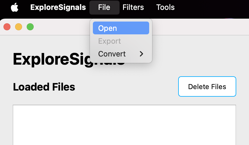
Files can be loaded using the File menu in the Explore Signals menu bar.

To load data:

Navigate to:
```
File > Open
```
Select one or multiple ExG files to load.

Supported file formats include:
- .csv
- .bdf

The loaded files appear in the Loaded Files section.

If you are loading Mentalab Explore data from an _ExG.csv file, make sure that the corresponding _Meta.csv file is present in the same folder. This ensures that the data is loaded correctly.

If you want to visualize markers alongside the data, make sure that the corresponding _Marker.csv file is also present in the same folder.

These files are matched using the file name. If you need to rename the files, for example after exporting filtered data with Explore Signals, make sure that:

the file containing ExG data ends in _ExG.csv
the file containing markers ends in _Marker.csv
the file containing metadata ends in _Meta.csv

Loading files in Explore Signals

Applying filters

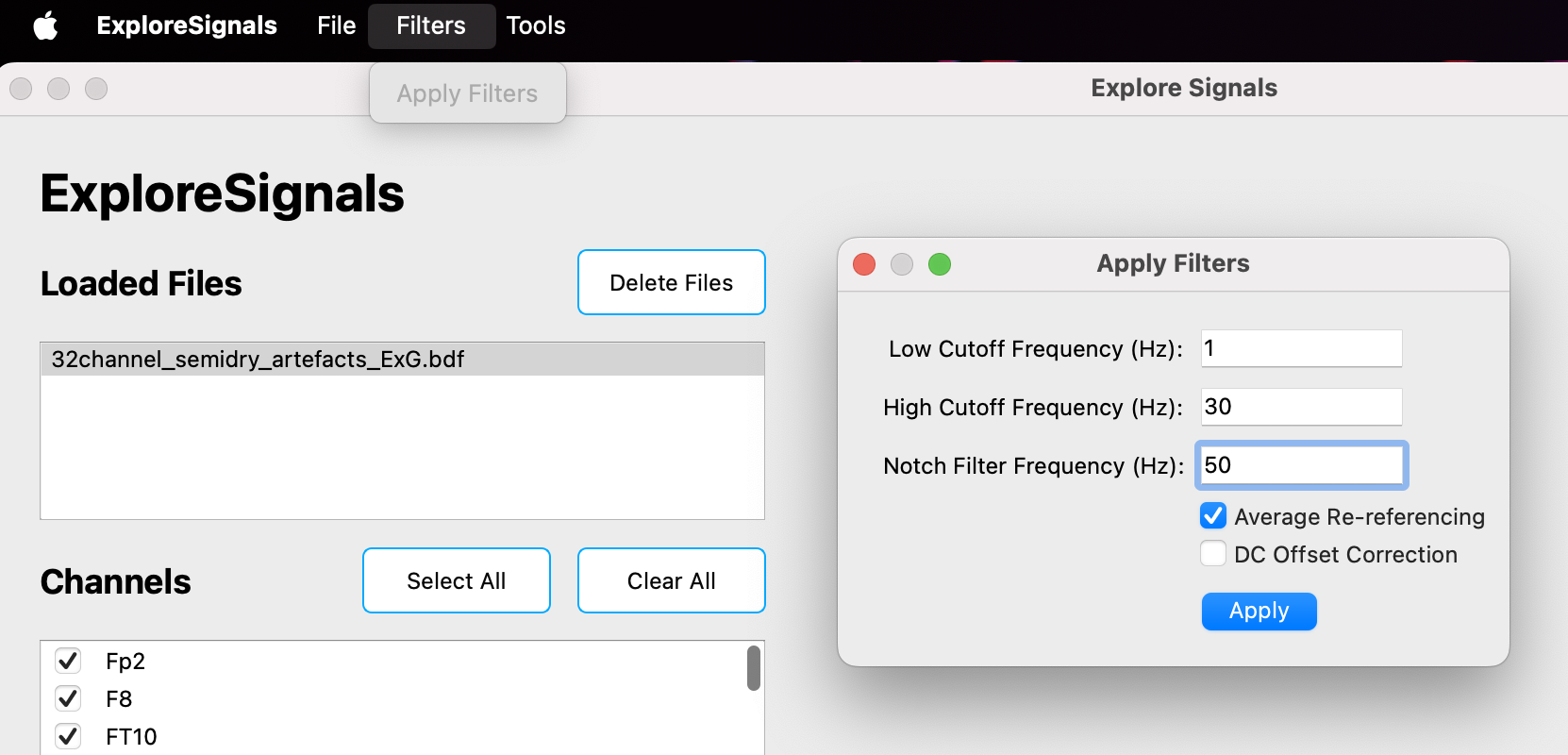
Filters can be applied from the Filters menu in the menu bar.

To apply filters:

Select the file you want to filter in the Loaded Files section.
Navigate to:
```
Filters > Apply Filters
```
Enter values for the filters you want to use.
Click Apply to filter the data.

The following filters are available:

High-pass filter
Low-pass filter
Notch filter, for example to remove 50 Hz or 60 Hz line noise
Re-referencing options
DC offset correction

The filtered data is added to the Loaded Files section. Its name is based on the original file name and metadata about the applied filters.

Filtering data in Explore Signals

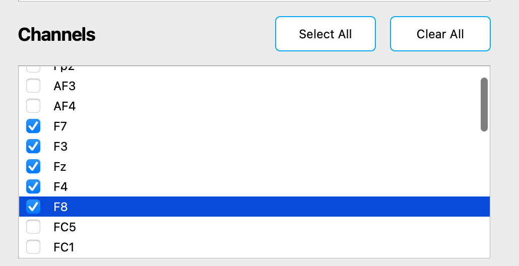
Channel selection

To enable or disable channels for visualization:

Select a file in the Loaded Files section.
Check or uncheck channels in the Channels section.
Use one of the visualization actions.

To quickly enable or disable all channels, use the Select All and Clear All buttons above the Channels section.

Selecting channels in Explore Signals

Visualization options

Click the corresponding button to visualize the selected data.

Use the interactive toolbar above the plots to zoom, pan, and explore plots in detail.

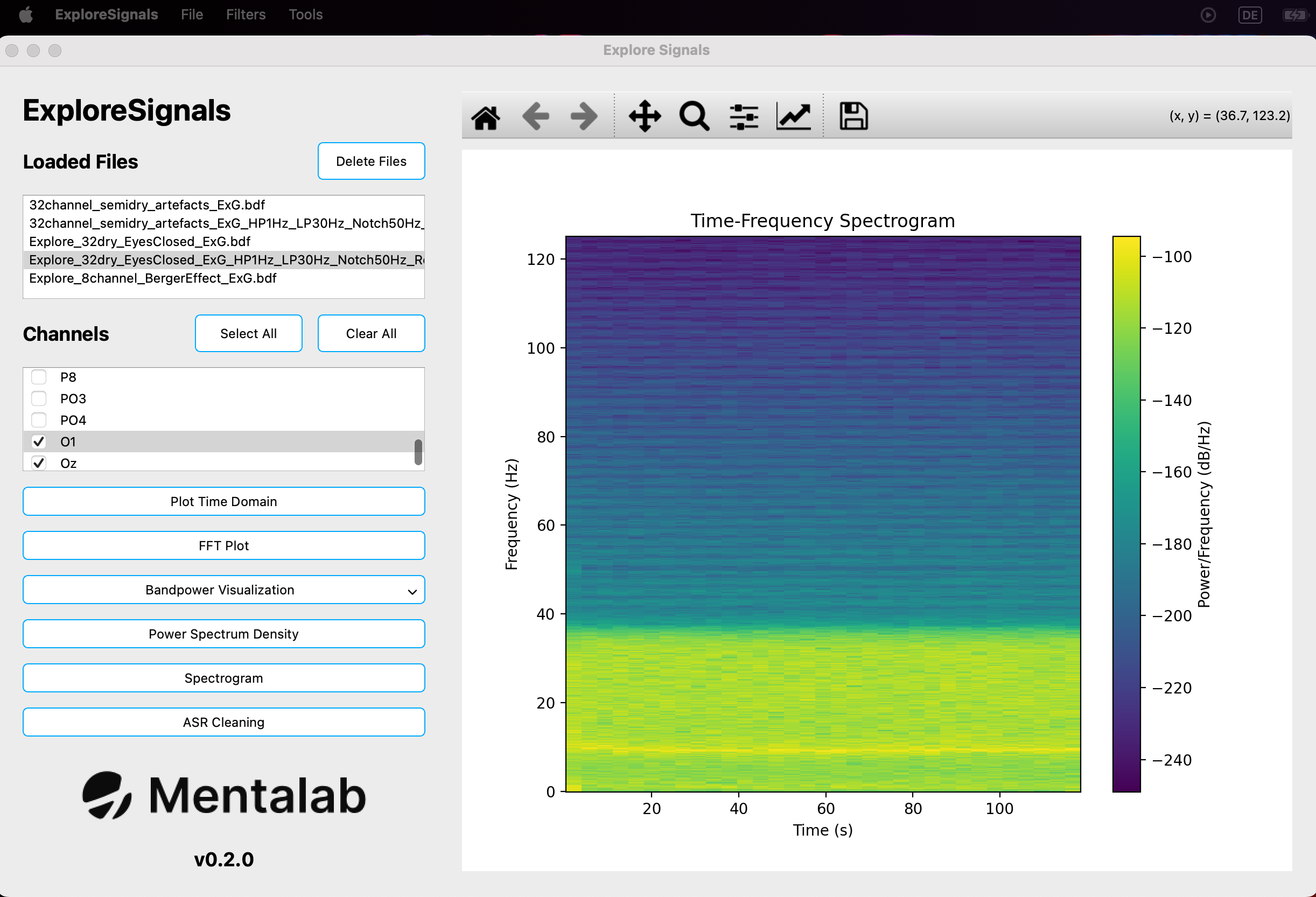
Time-domain plot

Use Plot Time Domain to view the raw signal over time.

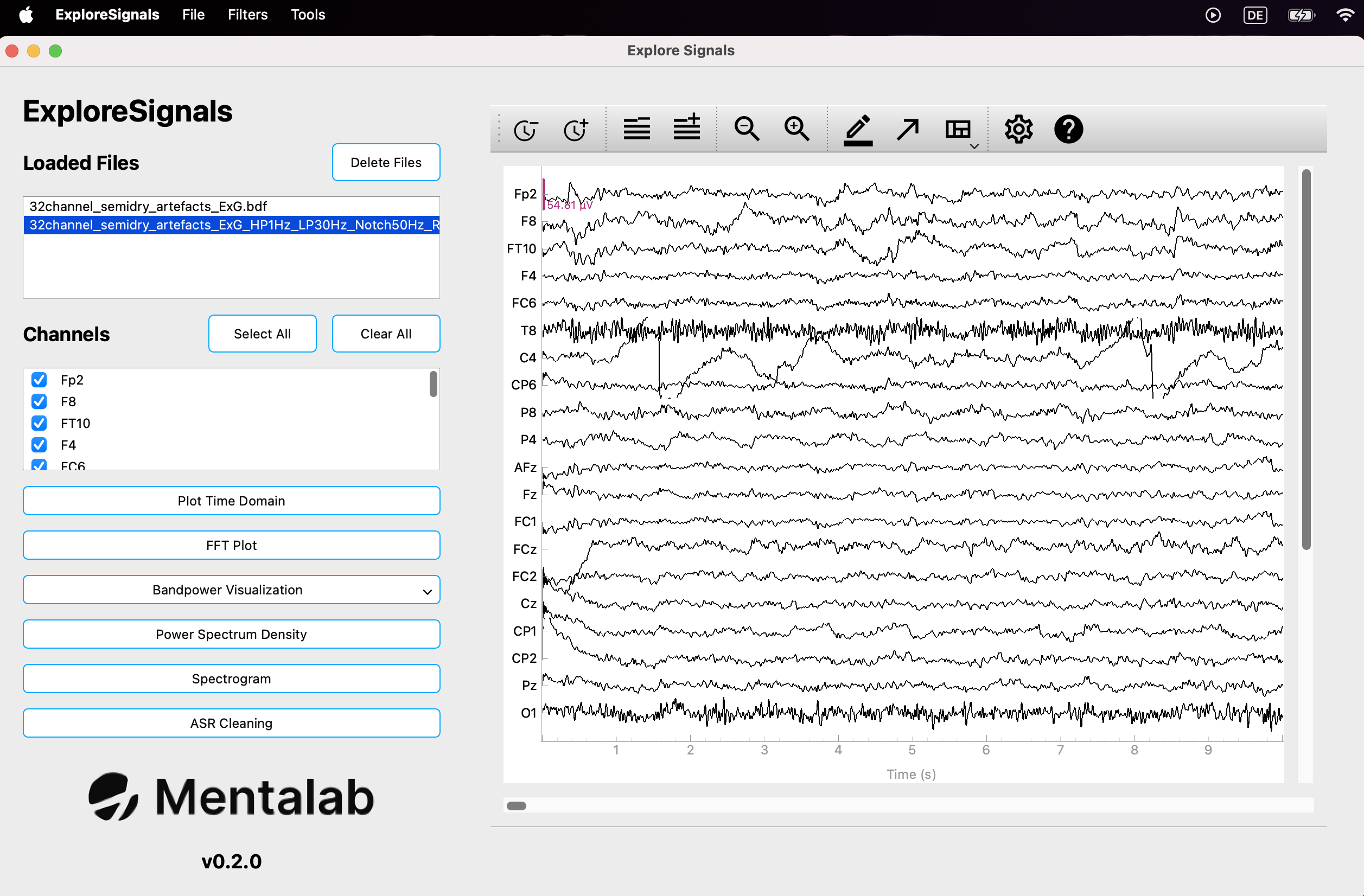
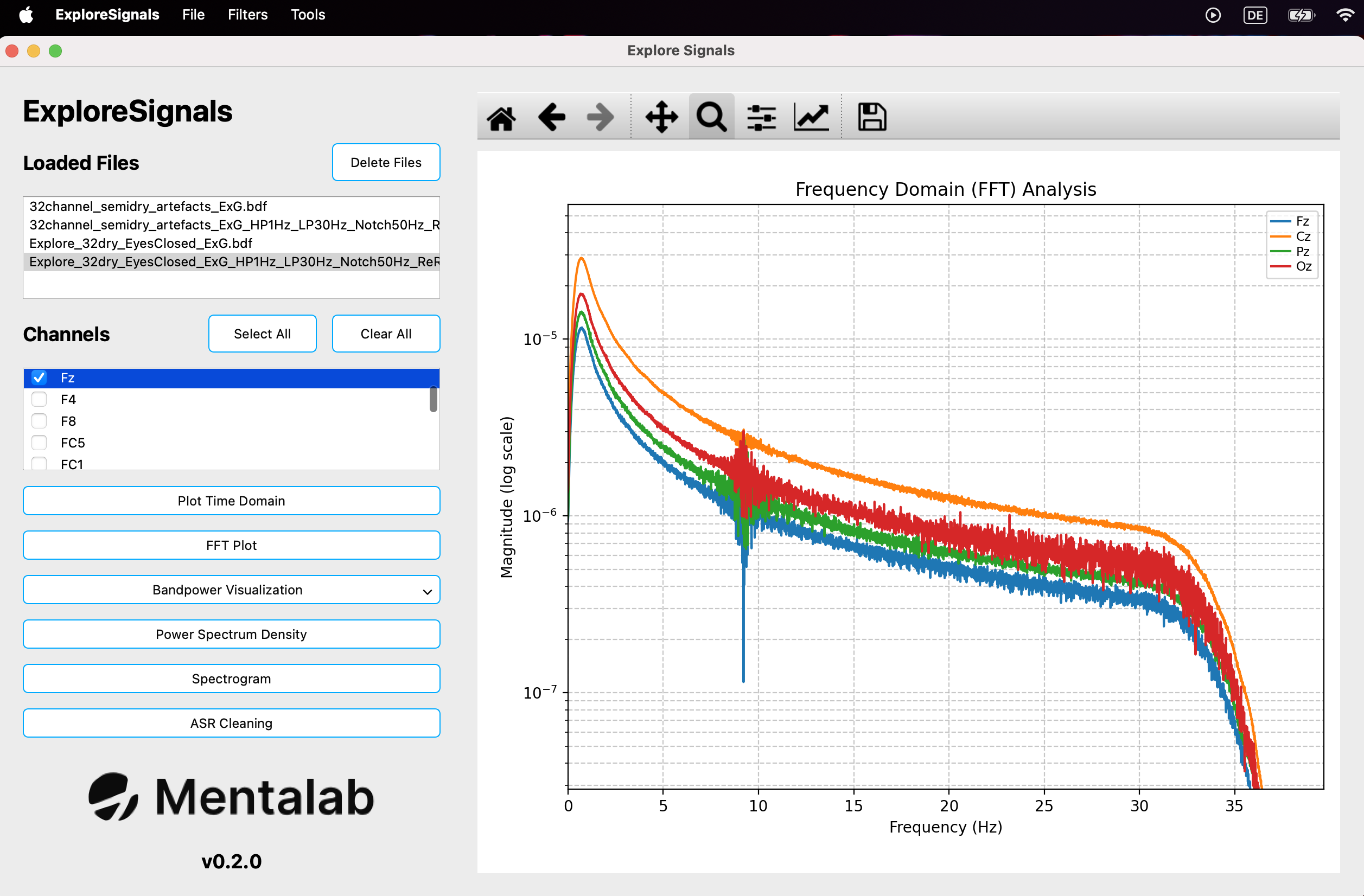
Example of visualizing signals over time in Explore Signals.

Time-domain visualization in Explore Signals

FFT plot

Use FFT Plot to visualize frequency content using the Fast Fourier Transform.

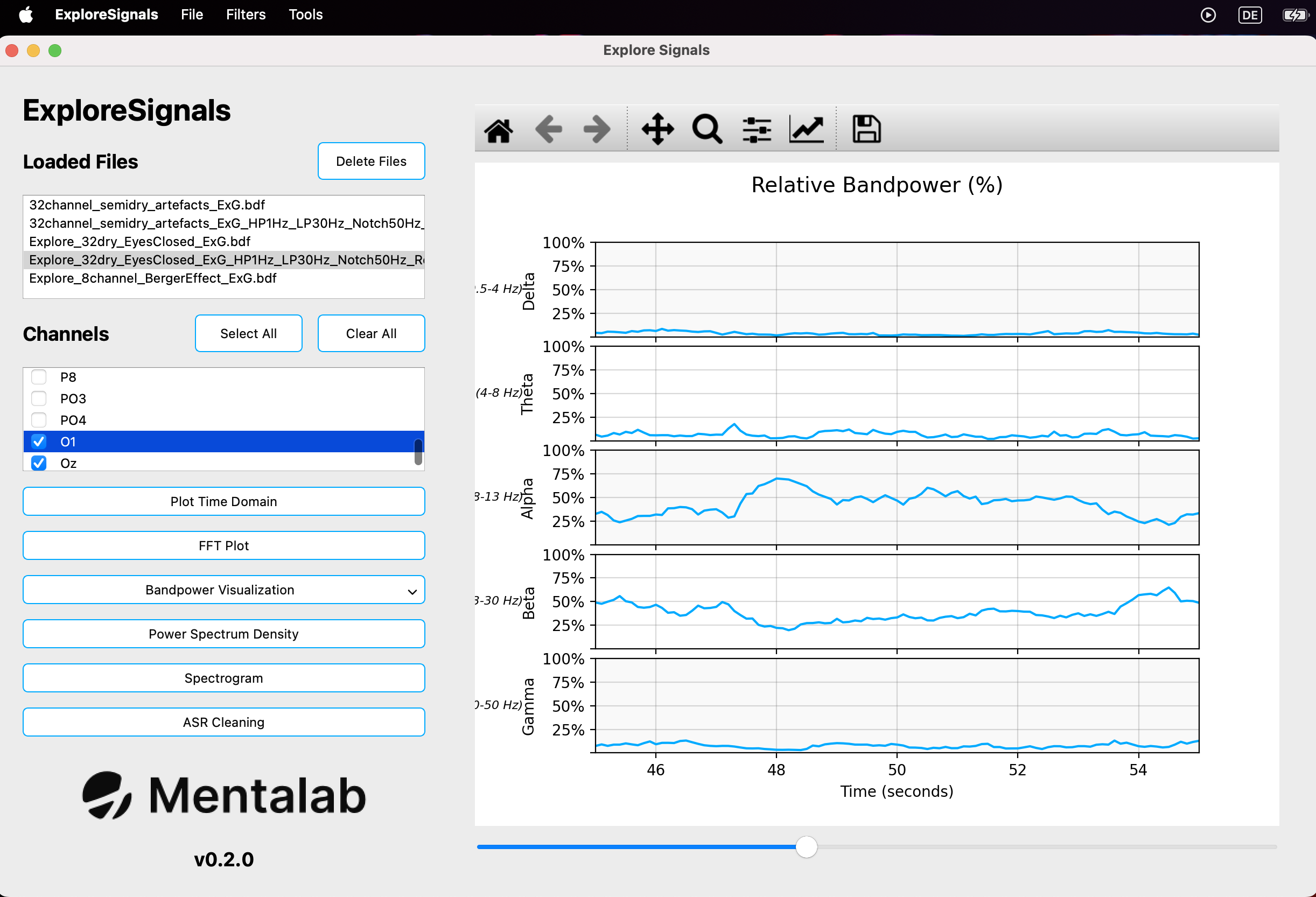
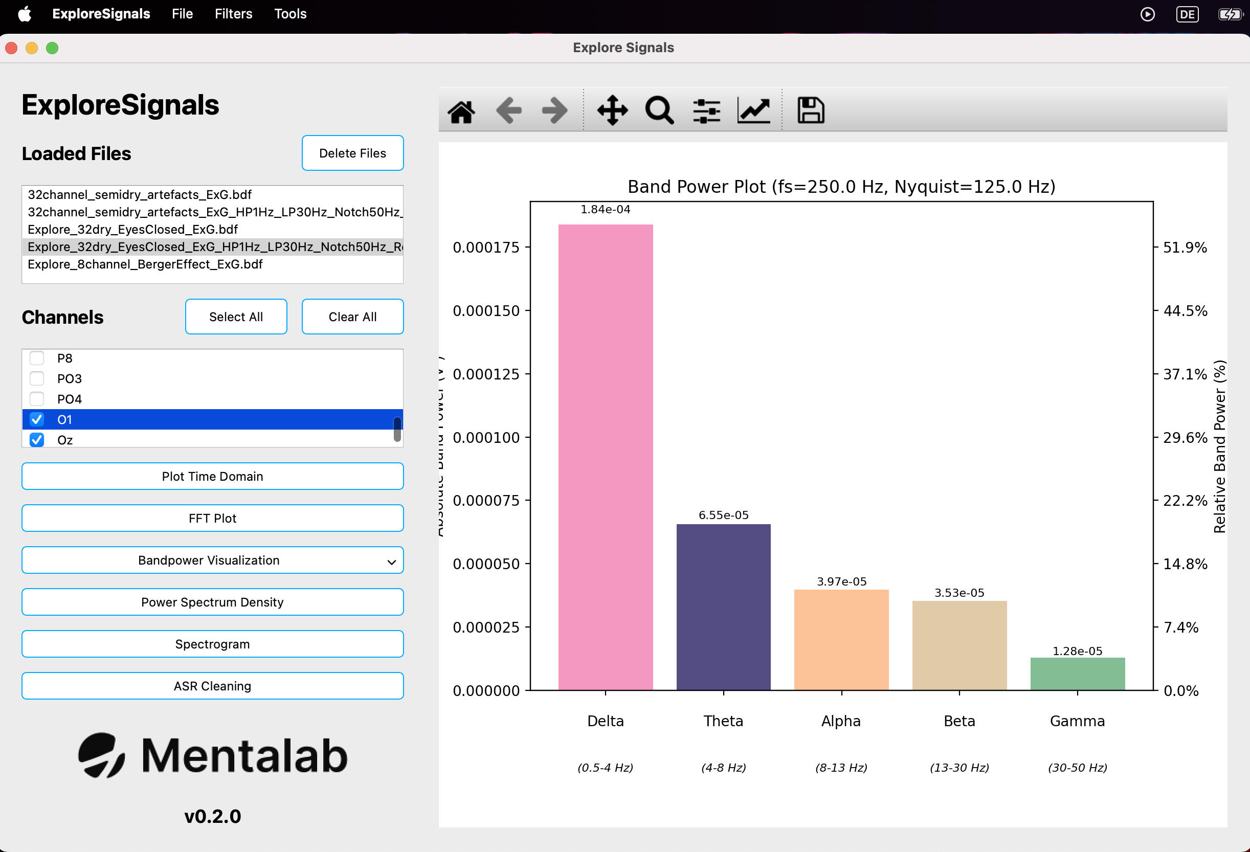
Visualizing the FFT of loaded data as a magnitude-over-frequency plot

Bandpower visualization

Use Bandpower Visualization to show power in defined frequency bands:

Delta
Theta
Alpha
Beta
Gamma

The plots show the average for the selected channels.

When clicking Bandpower Visualization, two visualization options are available.

Time domain

The time-domain bandpower plot visualizes power in the frequency bands over time.

For this plot, bandpower is calculated on 1 s windows with 0.1 s between each calculated sample.

Example of a bandpower over time plot in Explore Signals.

Visualizing power over time in the different frequency bands of a recording

Bars

The bar plot visualizes power in the frequency bands for the entire recording.

Example of a bandpower bar plot in Explore Signals.

Visualizing power in the different frequency bands of a recording as a bar plot

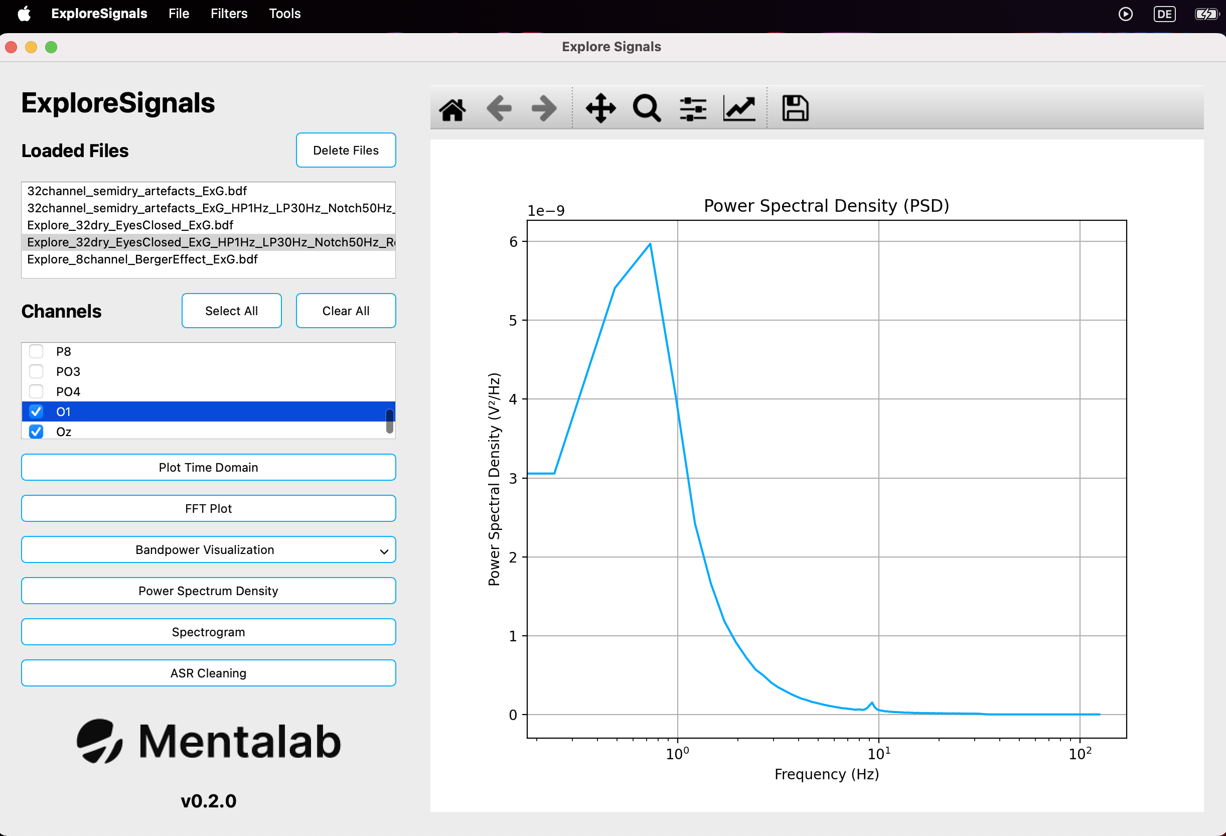
Power Spectrum Density

Use Power Spectrum Density to analyze power distribution over frequency.

The plot shows the average for the selected channels.

Example of a Power Spectrum Density plot in Explore Signals.

Visualizing the Power Spectrum Density of loaded data

Spectrogram

Use Spectrogram to display power as a function of time and frequency.

The plot shows the average for the selected channels.

Example of a spectrogram plot in Explore Signals.

Visualizing the spectrogram of loaded data

ASR cleaning

Use ASR Cleaning to apply Artifact Subspace Reconstruction to the data and visualize the cleaned signal alongside the original signal.

For more details, refer to the section on ASR.

Changing the settings before applying ASR

Comparing original data to cleaned data after applying ASR

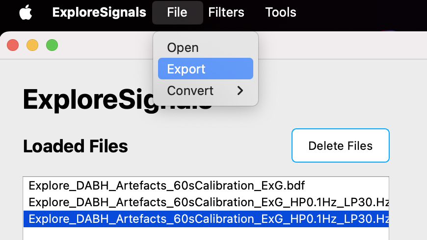
Exporting data

Original and processed data can be exported from the File menu in the menu bar.

To export data:

Select the file you want to export in the Loaded Files section.
Navigate to:
```
File > Export
```
Choose the file name.
Select the output file format.

Supported export formats include:
- .csv
- .bdf

Exporting data in Explore Signals

Artifact Subspace Reconstruction

Artifact Subspace Reconstruction, or ASR, is used to remove artifacts from EEG data.

The ASR implementation in Explore Signals is based on parts of the open-source clean_rawdata plugin for EEGLAB.

If you plan to apply ASR and work with cleaned data, make sure you understand the method and its limitations. ASR may remove signal together with artifacts and performs better on certain types of data.

ASR requires a calibration window. This should be a section of the data with as few artifacts as possible, ideally none.

Keep this in mind when selecting:

calibration window length
calibration start time

The algorithm is recommended for EEG signals. Output for other biosignals may be worse, for example if more signal than artifact is removed from the data.

Another factor to consider is the number of channels. ASR requires multiple channels to clean signals effectively. Research suggests that ASR can achieve effective artifact removal for standard 20-channel EEG[1].

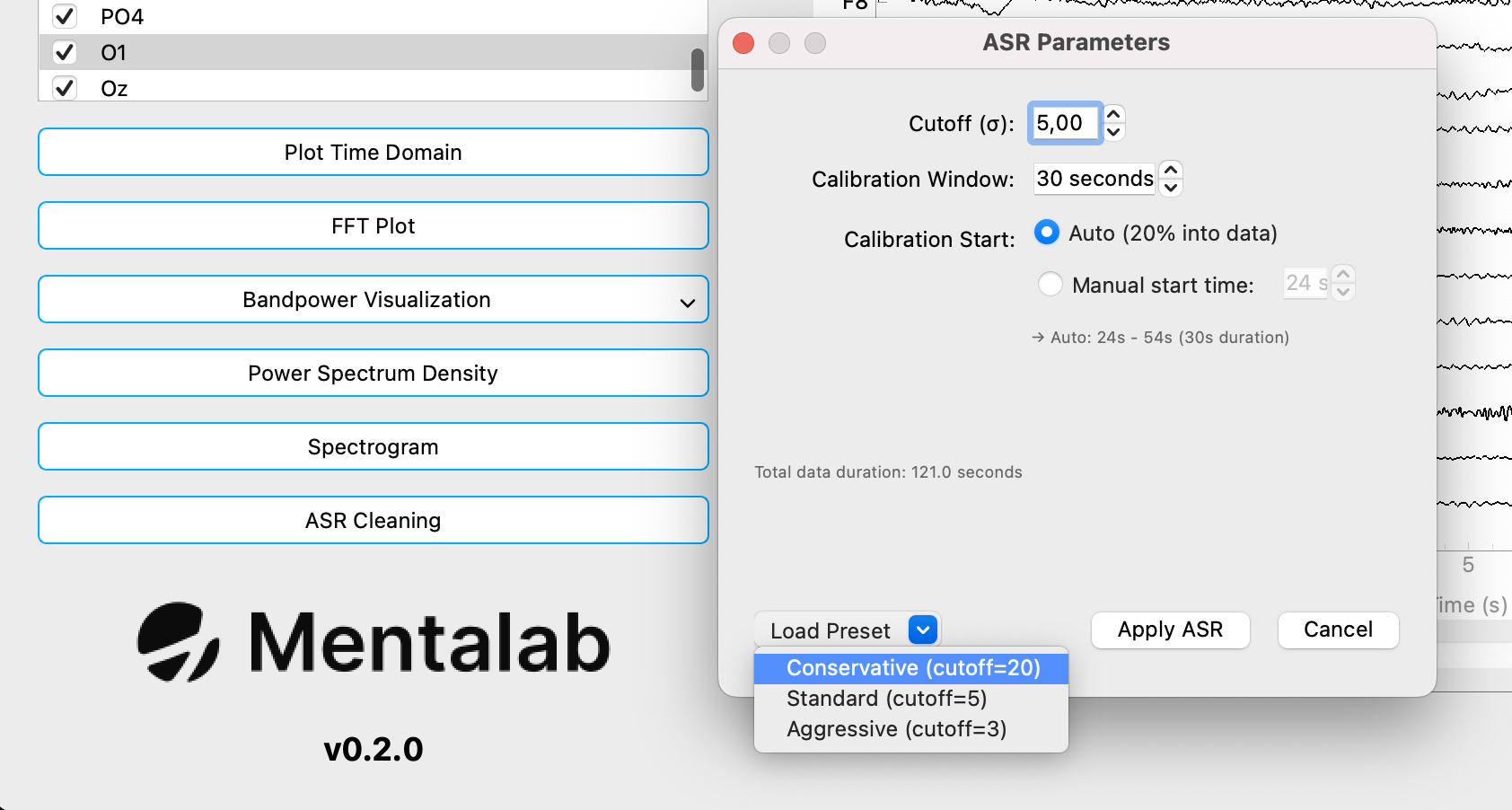
Standard deviation cutoff

The Cutoff field in the ASR pop-up refers to the standard deviation cutoff applied during cleaning.

This cutoff determines the thresholds used, relative to the calibration data, for recognizing portions of the data as artifacts.

A lower cutoff causes more data to be recognized as artifacts.
A higher cutoff causes less data to be recognized as artifacts.

The available presets are:

3.0 — aggressive
5.0 — standard and default in Explore Signals
20.0 — conservative and default in EEGLAB’s clean_rawdata plugin

Going below a cutoff of 3.0 is not recommended and is blocked by Explore Signals.

Calibration window

The Calibration Window determines the size of the data window used for calibration.

The default and minimum value is:

30.0 s

For a cutoff of 20.0, the recommended calibration window is:

60.0 s

Calibration start

The Calibration Start determines the beginning of the calibration window.

The default setting is Auto. This automatically places the start of the calibration window at 20% into the recording.

For example, if:

the recording is 120.0 s
the calibration window is 30.0 s
Auto is selected for Calibration Start

then the calibration window is placed from 24.0 s to 54.0 s.

Alternatively, you can manually choose the start of the calibration window by selecting Manual start time and changing the corresponding field to the desired starting second.

Applying ASR to a loaded file

To clean data using ASR:

Load a file.
Select it in the Loaded Files section.
Click ASR Cleaning.
Adjust the ASR parameters in the pop-up.
Optional: click Load Preset to load a recommended preset.

Available presets are:

Aggressive
- Cutoff: 3.0
- Calibration window: 30 s
Standard
- Cutoff: 5.0
- Calibration window: 30 s
Conservative
- Cutoff: 20.0
- Calibration window: 60 s

When you are finished changing the parameters, click Apply ASR.

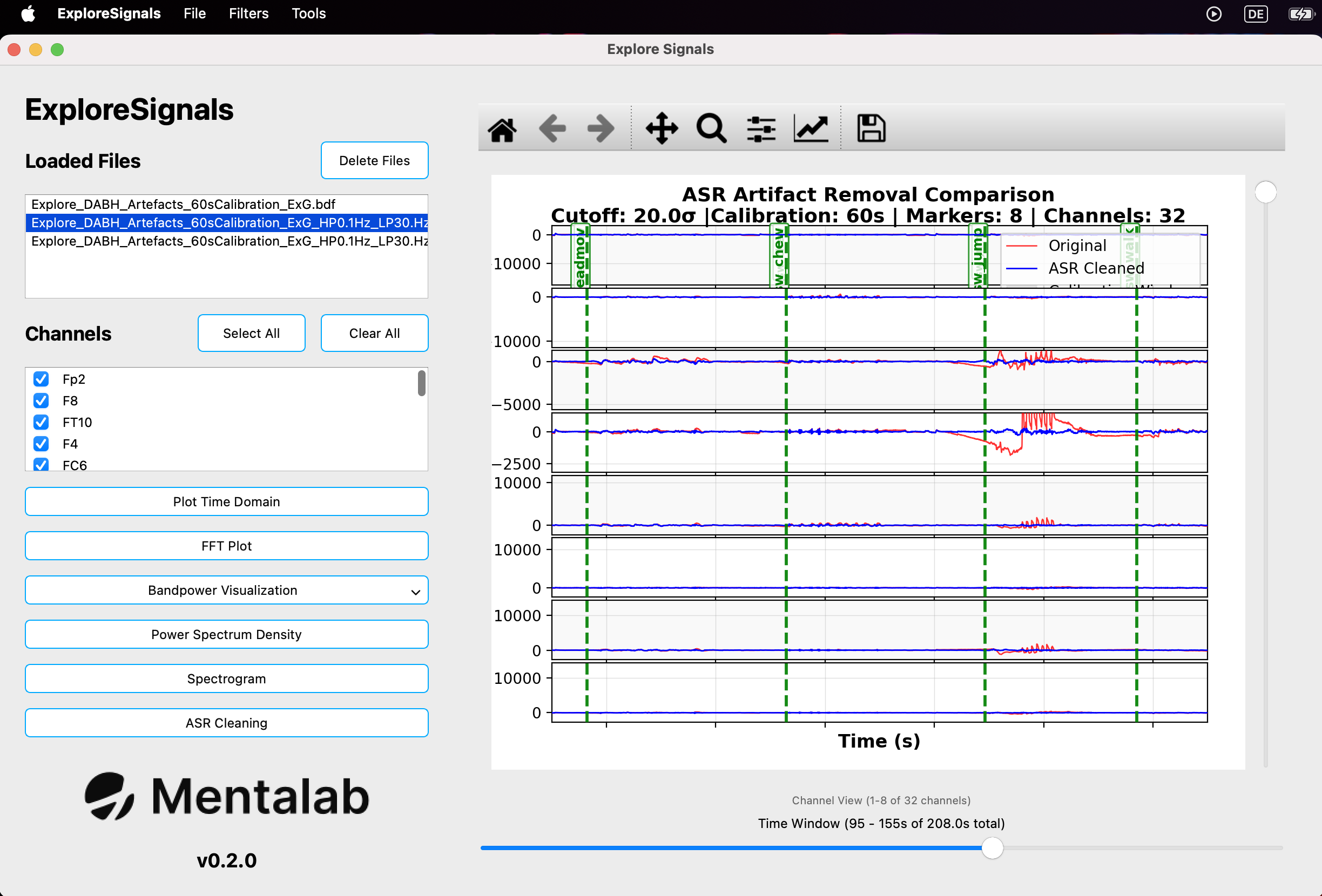
Explore Signals cleans the data and then opens a comparison view showing the cleaned data and the original data.

The ASR implementation applies a high-pass filter internally to correct for drift. The resulting cleaned signal is also zero-mean. If the original data is not filtered or zero-mean, the cleaned signal may not appear overlaid with the same baseline as the original signal.

The cleaned data is added to the Loaded Files section and can be visualized and analyzed like other loaded data.

Converting and repairing recordings

Converting to and from CSV and BDF

To convert an existing recording from .csv to .bdf or from .bdf to .csv:

Load the file you want to convert.
Export it to the other format.

Converting to EEGLAB dataset

Recordings in .csv, .edf, or .bdf format can be converted to .set files compatible with MATLAB’s EEGLAB plugin.

To convert recordings to EEGLAB datasets:

Navigate to:

File > Convert > Convert files to EEGLab

Select the folder containing the .edf or .bdf files to convert.

The .set files are created in a subfolder named datasets inside the selected directory.

To convert recordings from .csv format, the respective _Meta.csv file must be present in the same folder.

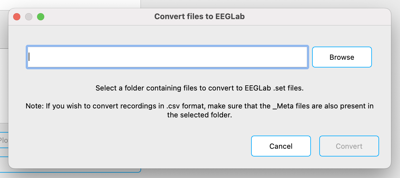
Convert recordings to EEGLAB datasets

Recordings in .csv and .bdf format can be converted to EEGLAB .set files.

Converting from BIN

You can convert binary files from the Explore device internal memory, in .BIN format, to .csv or .bdf files.

To convert a .BIN file:

Navigate to:

File > Convert > Convert .BIN to .csv or .bdf

Select the binary file to convert.
Select the folder where the converted files should be saved.
Select the output file format.

Converting to .csv generates four files:

_ExG.csv
_ORN.csv
_Marker.csv
_Meta.csv

Converting to .bdf generates two files:

_ExG.bdf
_ORN.bdf

Markers are written to the ExG file.

The data is written in BDF+ format using 24-bit resolution, as opposed to EDF or EDF+.

If you change the device sampling rate or channel mask during recording, conversion creates a new .csv or .bdf file for the ExG data. The file name includes the selected file name plus the time at which the setting changed.

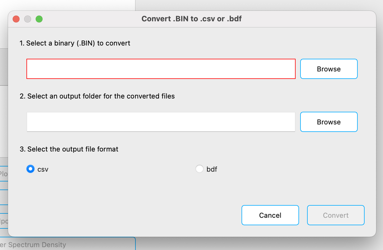
Convert BIN recordings in Explore Signals

Recordings from the Explore device internal memory can be converted from binary format to .csv or .bdf.

Repairing CSV recordings

If packets are dropped during recording with explorepy or Explore Desktop, the binary file from the Explore device can be used to repair the recorded .csv file.

To repair a recorded .csv file:

Place the .csv file and the matching .BIN file in the same folder.
Navigate to:
```
Tools > Repair ExG .csv with .BIN
```
Select the .csv file to repair.
Click Repair.

The repaired file is placed in the same folder as the selected file. It is named like the selected file, but with _recovered_ExG added to the file name.

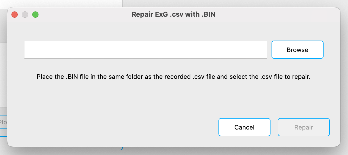
Repair CSV recording in Explore Signals

Recordings made with explorepy or Explore Desktop that may have missing samples can be repaired using a matching binary file from the Explore device internal memory.

Support

For more information or support, contact support@mentalab.com.

References

[1] Chang, Chi-Yuan, et al. "Evaluation of artifact subspace reconstruction for automatic artifact components removal in multi-channel EEG recordings." IEEE Transactions on Biomedical Engineering 67.4 (2019): 1114-1121.