Real-time Spectrogram
Introduction
The spectrogram of a signal contains the magnitude of the frequencies of the signal over time, meaning it contains three dimensions: time, frequency and magnitude. This data can be plotted as an image that is essentially a heatmap of frequencies over time.
This example application shows how this can be achieved with real-time updates using the Mentalab Explore device, explorepy and a few other dependencies.
Requirements
- Mentalab Explore
- A Python 3 installation, we strongly recommend using Anaconda to install Python and using version 3.12
Setting up the environment and dependencies
- Set up an environment with Python version 3.12 with conda and activate it:
conda create -n spectrogram python=3.12
conda activate spectrogram
- Install liblsl, which is required by explorepy, via conda-forge:
conda install -c conda-forge liblsl
- Install the other dependencies via pip:
pip install explorepy glfw vispy scipy numpy
Running the example
Adapting the script to your needs
The code for this example (real_time_spectrogram.py) can be found in the examples folder of the GitHub repository for explorepy: https://github.com/Mentalab-hub/explorepy/
You can run the script in the environment you’ve set up by calling python -m real_time_spectrogram and supplying command line arguments according to your needs:
| argument | description | required | default |
|---|---|---|---|
-n, --device_name |
The name of your device, i.e. Explore_ABCD | yes | - |
-sr, --sampling_rate |
The sampling rate to set the device to | no | None / current device sampling rate |
-uw, --update_window |
The time between updates of the plot (in seconds) | no | 0.1s for mode overlapping, 0.5s otherwise |
-tw, --time_window |
The total time window displayed in the plot (in seconds) | no | 10s |
-usb |
Whether to connect via USB | no | False |
-fn, --notch |
The frequency to use for the notch filter | no | None |
-fbp, --bandpass |
The frequencies to use for the bandpass filter | no | None |
-m, --drawing_mode |
The mode used for drawing the plot (options: moving_fft, moving_stft, overlapping) |
no | moving_fft |
For example, to run the script with default values for the device Explore_ABCD:
python -m real_time_spectrogram -n Explore_ABCD
An example that uses every option:
python -m real_time_spectrogram -n Explore_ABCD -sr 500 -uw 0.5 -tw 20 -usb -fn 50.0 -fbp 3.0 30.0 -m overlapping
This call will…
- set the sampling rate to 500Hz
- set the update window to 0.5s
- set the time window to 20s
- tell the script to connect via USB
- add a Notch filter for the frequency 50Hz
- add a Bandpass filter with the low cutoff frequency 3.0Hz and high cutoff frequency 30.0
- use the drawing mode
overlapping
In addition to the command line arguments, a configuration dictionary is defined in the code and can be adapted (in if __name__ == '__main__').
config = {"window": "hann", "nperseg": 128, "noverlap": 0}
The values in this dictionary are passed to scipy’s stft method to fine-tune how the STFT (Short-time Fourier Transform) is calculated. The config can be set to None (config = None) to use scipy’s default values for the STFT.
The plot will only show up after the buffer has been filled up once, meaning the window will only appear after update_window seconds for the modes moving_fft and moving_stft or after time_window seconds for the mode overlapping.
Depending on the chosen parameters, the result of the STFT (or joined together results) may lead to a stretched out plot. For example, if the sampling rate is set to 1000Hz, the drawing mode is moving_fft, the update window 1s and the time window 10s, the plot will hold 10 pixels on the x-axis (10/1 = 10) but 500 on the y-axis (1000/2 = 500). In order to mitigate this, the plot’s camera is manipulated in the script to make the plot appear square instead of stretched out:
self.plot.camera.aspect = self.img.shape[0] / self.time_window
Commenting out this line will show the original aspect ratio of the plot.
Additionally, a frequency cut-off for the y-axis can be supplied to the plot (f_cutoff):
rt_spectrogram = SpectrogramPlot(device_sr=dev_sr,
                                 update_window=uw,
                                 time_window=tw,
                                 mode=args.drawing_mode[0],
                                 colormap="viridis",
                                 config=config,
                                 f_cutoff=70)
The default cut-off value if nothing is supplied is 70, this value determines how many rows of the image should be plotted.
Drawing modes
The logic for all drawing modes is the same, either the STFT or the FFT (Fast Fourier Transform) is calculated on a buffer containing channel values and its result is used to update a numpy array that is then interpreted as an image to be plotted.
overlapping
In this mode, the STFT is calculated for the entire time_window. The STFT is recalculated every update_window seconds on the last time_window seconds of data. In order to do this, the first update_window * device_sr many samples are dropped from the buffer every update. The result of the STFT is used to overwrite the entire numpy array that makes up the plot.
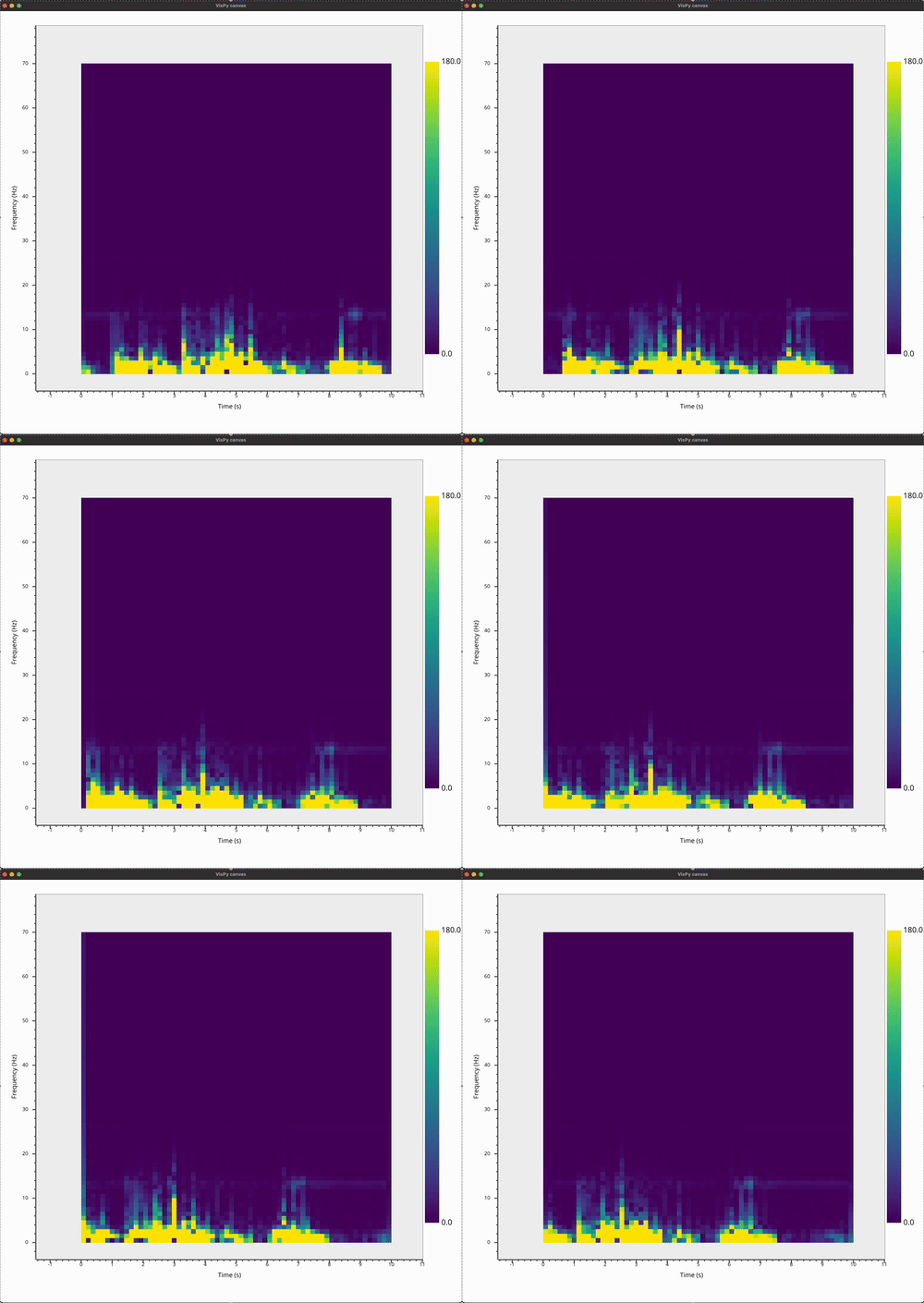
moving_fft
In this mode, the FFT is calculated on the update_window. Afterwards, the buffer is cleared and fills up until update_window * device_sr many values are inside before the FFT is recalculated. Every result is treated as a column of pixels for the resulting plot and updates the column of values in the numpy to the right of the last updated column, building up the plot slice by slice. Additionally, a rudimentary swiping line is drawn to the right of the latest pixel column. When right edge of the plot is reached, it starts updating from the left edge again.
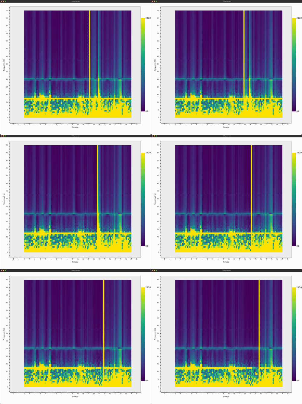
moving_stft
This mode can be seen as a hybrid of the other two modes. It calculates the STFT on the update_window and updates multiple columns in the numpy array with its result, updating the plot chunk by chunk.
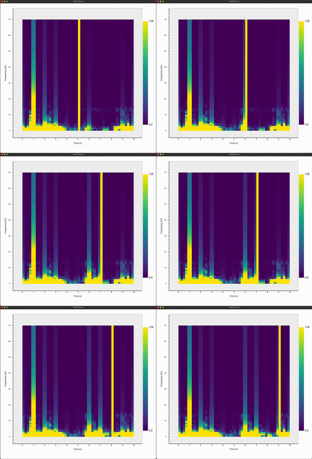
Keyboard interactions
The cut-off value for the plot can be increased or decreased by pressing the up or down key on the keyboard. This value corresponds to the colour at the top of the colourmap to the right, any values coming from the STFT or FFT that are higher than this value will be displayed with the same colour as values at the cut-off.
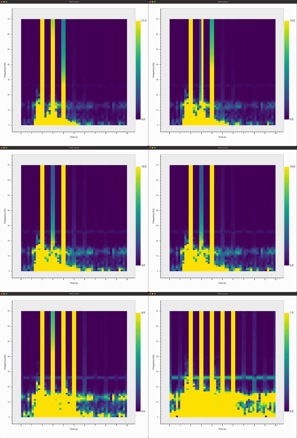
The colourmap for the plot can be changed in code and by default is set to “viridis”. All available colourmaps can be cycled through by pressing the C key. The colourmap maps values from the STFT or FFT to a colour.
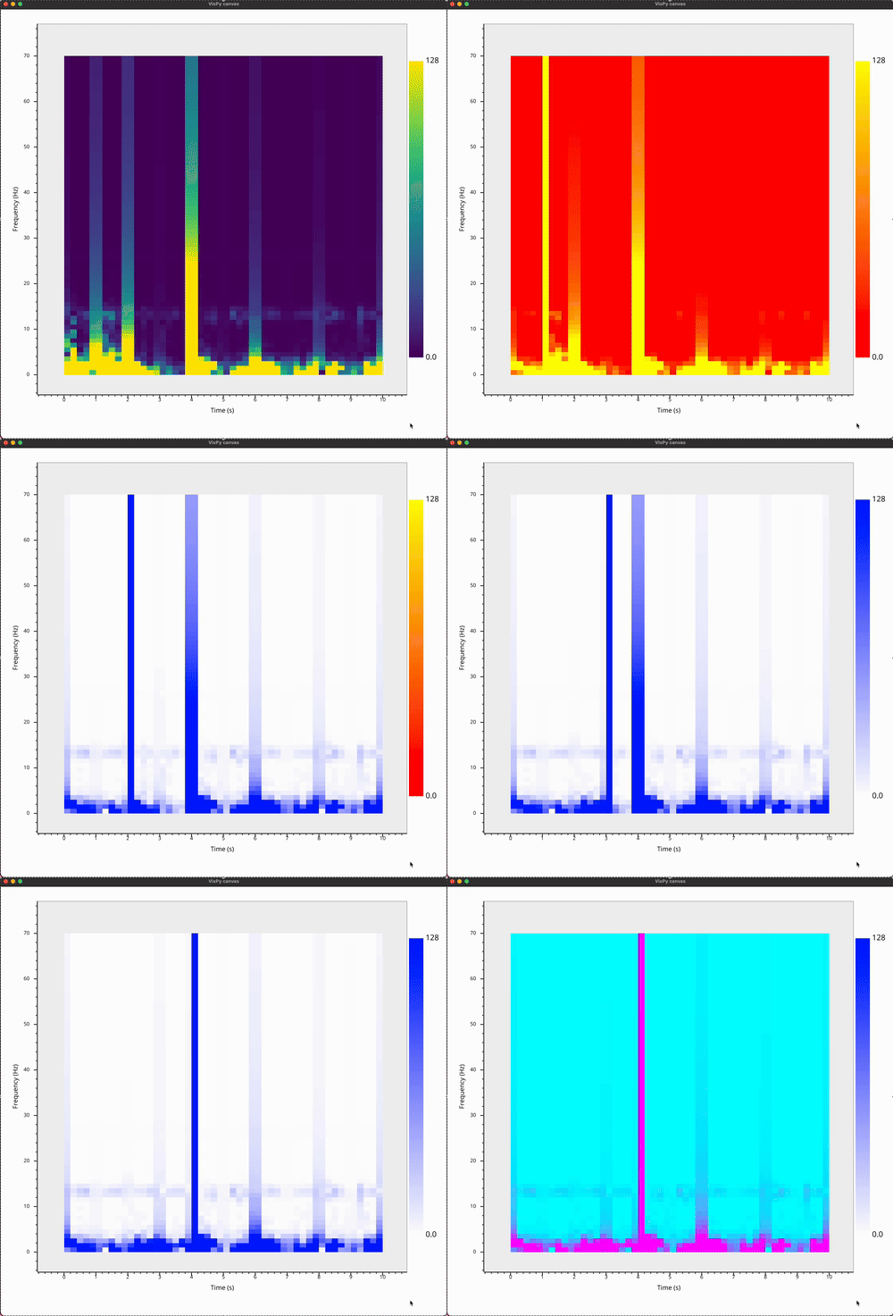
The drawing mode, maximum time window, update window and sampling rate all influence the frequency and time resolution of the plot.
Higher frequency resolution is achieved with longer buffers, which in turn can be achieved by increasing the time between updates for the modes moving_fft and moving_stft (since these modes calculate the STFT or FFT with update_window * device_sr many samples). For overlapping, this means increasing the time window (since the STFT is calculated every update_window seconds on time_window * device_sr many samples). This also means the frequency resolution can be improved with higher device sampling rates.
Higher temporal resolution is achieved with higher update rates. This can be achieved by reducing the time between calculations. For the modes moving_fft and moving_stft this corresponds to decreasing the update_window, for the mode overlapping this corresponds to decreasing the time_window. Increasing the sampling rate of the device can thus improve the temporal resolution without sacrificing resolution in the frequency axis.
Mouse interactions
The example uses vispy’s powerful plotting module to plot the spectrogram as an image. The plot uses a PanZoomCamera by default which - as the name suggests - allows the user to pan the plot using the click-and-drag gestures and zoom the plot using the scroll wheel.