Sleep EEG Analysis
Modern sleep science is fundamentally informed by ExG biosensors recording brain activity (electroencephalography, EEG), eye-movement activity (electrooculography, EOG), and muscle activity (electromyography, EMG) to characterize the physiology of sleep.
Here, we demonstrate how EEG data recorded during a full night’s sleep using Mentalab Explore can be analysed with the free and open source yasa toolbox. We will perform automatic sleep staging by applying the yasa classifier [1] to EEG data, inspect band power in the EEG signal, and detect slow waves and sleep spindles. The application example follows the excellent yasa notebooks.
Data acquisition
Our volunteer recorded their sleep using an 8-channel Mentalab Explore device. The following montage was applied:
Channel Type    Electrode   Position
0       REF     adhesive    TP10 (right mastoid)
1       EOG     adhesive    above right eye
2       EOG     adhesive    outer canthus right eye
3       EMG     adhesive    submental (below chin)
4       EEG     dry         O2
5       EEG     dry         C2
6       EEG     dry         F2
7       EEG     adhesive    C1
8       EEG     wet         Fc1
Clip cables were used to connect to adhesive and dry electrodes. Dry electrodes use flexble brushes to establish connection. Impedances were not lowered after positioning the electrodes. Refer to our sleep recording protocol, for detailed reccomendations on preparation, data transfer, and on how to convert the recorded BIN file to .csv or .bdf files.
Sleep data analysis
Software preparation
First, we prepare a conda virtual Python environment to house our project.
- (Install anaconda)
- Create a virtual python environment using conda:
conda create -n myenv python=3.10 - Activate your conda environment:
conda activate myenv - Install the required packages:
pip install numpy mne yasa
Data processing
We then load the required packages in python.
import mne
import yasa
import numpy as np
import matplotlib.pyplot as plt
We will load a CSV file containing the sleep data recorded using Mentalab Explore and convert it to an mne raw data object. The code example expects data recorded at 250 Hz with an 8-channel device. It is important to note that mne expects data in Volt (V), whereas Mentalab Explore stores data in Microvolt (µV).
ch_names = ['EOG-above', 'EOG-canthus', 'EMG-chin', 'Dry-O2', 'Dry-C2', 'Dry-F2', 'Sticky-C1', 'Wet-Fc1']
data = np.loadtxt("./data/wiki-sleep-analysis-data/Mentalab-sleep-analysis_ExG.csv",skiprows=1,delimiter=',').transpose()[1:9]
sf = 250
ch_types = ["eog", "eog", "emg", "eeg", "eeg", "eeg", "eeg", "eeg"]
info = mne.create_info(ch_names = ch_names, sfreq = sf, ch_types = ch_types)
raw = mne.io.RawArray(data, info)
raw.apply_function(lambda x: x * 1e-6) # scale muV to V
Next, we apply a band-pass filter with a low cutoff of 0.1 Hz and a high cutoff of 40 Hz.
raw.filter(0.1, 40) # Apply a bandpass filter from 0.1 to 40 Hz
Detecting sleep stages
Next, we apply the yasa sleep stage classification algorithm [1]. The only required input is one channel of EEG data. While the algorithm can additionally receive one channel of EOG data, one channel of EMG data, and the age and gender of the participant, these additional inputs are not required. In fact, the EEG channel accounts for almost all of the classifier’s performance [1].
sls = yasa.SleepStaging(raw, eeg_name="Sticky-C1")
y_pred = sls.predict() # Get the predicted sleep stages

hypno = yasa.Hypnogram(y_pred) # Getting a hypnogram for later
hypno_int = yasa.hypno_str_to_int(y_pred)
hypno_up = yasa.hypno_upsample_to_data(hypno=hypno_int, sf_hypno=(1/30), data=data, sf_data=sf)
Inspecting band power
Sleep stages are typically associated with brain activity in specific EEG frequency bands. For instance, N3 sleep is defined by slow waves in the delta band, whereas REM sleep is associated with increased alpha frequency power. We compute the relative power for each sleep stage (Wake, N1, N2, N3, REM) in six common frequency bands (delta, theta, alpha, sigma, beta).
data_filt = raw.get_data() * 1e6
data_c1_uV = data_filt[6]
bandpower_stages = yasa.bandpower(data_c1_uV, sf = 100, win_sec=4, relative=True, hypno=hypno_up, include=(0, 1, 2, 3, 4))
bandpower_avg = bandpower_stages.groupby('Stage')[['Delta', 'Theta', 'Alpha', 'Sigma', 'Beta', 'Gamma']].mean()
bandpower_avg.index = ['Wake', 'N1', 'N2', 'N3', 'REM']
Inspecting the relative band power, we observe increased delta and decreased theta activity in N3 sleep compared to being awake. Further, increased alpha activity is observed in N1 and REM sleep compared to the deeper N2 and N3 sleep stages.
print(bandpower_avg)
      Delta     Theta     Alpha     Sigma     Beta      Gamma
Wake  0.689047  0.252754  0.041008  0.013561  0.003619  0.000011
N1    0.805558  0.156776  0.026298  0.008975  0.002385  0.000009
N2    0.860466  0.122272  0.011644  0.004467  0.001142  0.000010
N3    0.934785  0.058335  0.004424  0.001922  0.000521  0.000014
REM   0.848217  0.115585  0.025746  0.008503  0.001937  0.000010
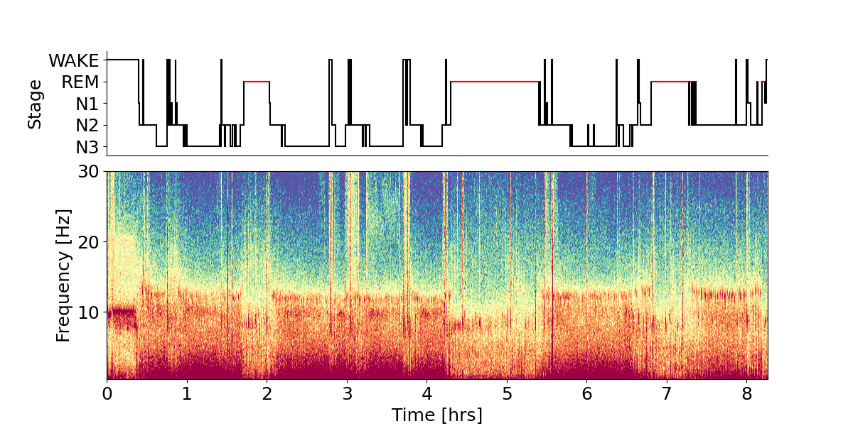
Spectrogram and hypnogram
A hypnogram is a visual representation of the sleep stages over the course of the night. In Figure 1 the hypnogram is combined with a spectrogram displaying the frequency content over time. The hypnogram exhibits a typical pattern of deeper sleep stages in the first half of night and longer REM stages in the second half of the night. The spectrogram reveals power in specific frequency bands that the sleep stages are associated with. Note that usually, clinical sleep recordings are tagged by trained professionals according to the AASM guidelines (American Academy of Sleep Medicine), whereas the hypnogram shown here is based on the classifier’s automatic sleep detection.
fig = yasa.plot_spectrogram(data_c1_uV, sf, hypno=hypno_up, fmax=30, cmap='Spectral_r', trimperc=5)
fig.show()
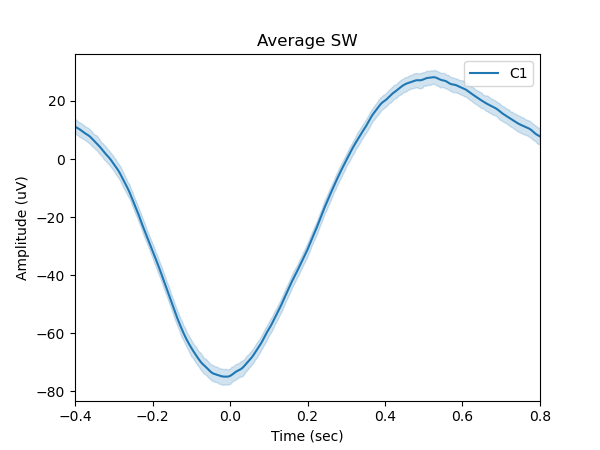
Slow wave and sleep spindles detection
Slow waves are a hallmark of the N3 sleep stage (also known as slow wave sleep) and, with frequencies between 0.5 and 3 Hz, are part of the delta frequency band. The yasa toolbox provides an slow wave detection algorithm (based on [2, 3]) that allows to inspect individual and averaged slow waves.
Calling the slow wave summary function yields an overview of the timing and properties of the detected slow waves.
sw = yasa.sw_detect(data_c1_uV, sf, hypno=hypno_up)
sw.summary()
        Start    NegPeak  MidCrossing    PosPeak        End  Duration  ValNegPeak  ValPosPeak         PTP       Slope  Frequency  Stage  Channel  IdxChannel
0     1579.324   1579.600     1579.860   1580.076   1580.400     1.076 -110.009728   70.868551  180.878280  695.685692   0.929368      2  CHAN000           0
1     1833.080   1833.328     1833.560   1833.844   1834.144     1.064  -43.119826   50.537236   93.657062  403.694232   0.939850      2  CHAN000           0
2     1834.144   1834.452     1834.736   1834.896   1835.060     0.916  -64.484388   26.909410   91.393798  321.809148   1.091703      2  CHAN000           0
3     1895.844   1896.224     1896.560   1896.808   1897.060     1.216  -55.624535   42.378489   98.003024  291.675667   0.822368      2  CHAN000           0
4     1935.872   1936.280     1936.700   1936.832   1936.984     1.112  -83.590539   10.574031   94.164569  224.201355   0.899281      2  CHAN000           0
..         ...        ...          ...        ...        ...       ...         ...         ...         ...         ...        ...    ...      ...         ...
966  29275.144  29275.496    29275.784  29276.000  29276.756     1.612 -123.916814   68.232216  192.149031  667.184134   0.620347      2  CHAN000           0
967  29276.756  29277.024    29277.292  29277.484  29277.780     1.024  -80.189417   37.322052  117.511469  438.475632   0.976562      2  CHAN000           0
968  29351.656  29351.996    29352.252  29352.468  29352.712     1.056  -80.538877   63.521518  144.060395  562.735919   0.946970      2  CHAN000           0
969  29353.720  29354.168    29354.448  29354.660  29354.980     1.260  -60.494303   36.531033   97.025336  346.519058   0.793651      2  CHAN000           0
970  29444.048  29444.400    29444.704  29444.924  29445.248     1.200 -166.011564   85.047673  251.059236  825.852751   0.833333      2  CHAN000           0
Figure 2 shows the average slow wave, computed from 971 detected slow wave events.
sw.plot_average(time_before=0.4, time_after=0.8, center="NegPeak");
plt.legend(['C1'])
plt.show()
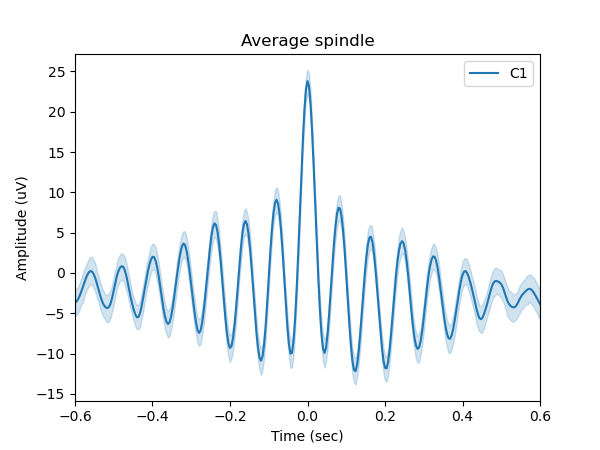
Sleep spindles are a short oscillatory bursts that typically occur during N2 sleep and fall in the frequency range between 11 and 16 Hz. Using the same workflow as before we run the spindle detection algorithm (based on [4]). Calling the sleep spindle summary function yields an overview of the timing and properties of the detected sleep spindles.
sp = yasa.spindles_detect(data_c1_uV, sf)
sp.summary()
        Start       Peak        End  Duration   Amplitude        RMS  AbsPower  RelPower  Frequency  Oscillations  Symmetry  Channel  IdxChannel
0        8.720      8.864      9.396     0.676   56.961351  11.090094  2.100221  0.322695  11.315217           8.0  0.211765  CHAN000           0
1       53.476     53.532     54.152     0.676  147.736709  28.034810  2.648341  0.305501  12.936249           8.0  0.082353  CHAN000           0
2     1399.952   1400.424   1400.636     0.684   58.795353  11.988885  1.960096  0.266393  13.047958           8.0  0.686047  CHAN000           0
3     1444.672   1444.860   1445.176     0.504   49.023655  11.592732  2.043340  0.243198  13.838615           7.0  0.370079  CHAN000           0
4     1496.024   1496.072   1496.672     0.648   37.978448  10.030894  1.689857  0.238392  13.444519           8.0  0.073620  CHAN000           0
..         ...        ...        ...       ...         ...        ...       ...       ...        ...           ...       ...      ...         ...
519  29412.916  29413.096  29413.660     0.744   37.617005   8.592611  1.851378  0.323409  12.606909           8.0  0.240642  CHAN000           0
520  29418.196  29419.088  29419.892     1.696   73.779483  14.525022  2.380002  0.519697  12.552197          21.0  0.524706  CHAN000           0
521  29423.800  29425.016  29425.484     1.684   58.250863  11.203151  1.982496  0.389862  12.449155          21.0  0.720379  CHAN000           0
522  29451.216  29452.136  29452.268     1.052   46.337193  10.750559  2.002255  0.438899  12.765855          13.0  0.871212  CHAN000           0
523  29467.156  29467.684  29468.148     0.992   49.976640   9.770195  1.971178  0.429425  12.662866          12.0  0.530120  CHAN000           0
Figure 3 shows the average sleep spindle, computed from 524 detected spindle events.
sp.plot_average(time_before=0.6, time_after=0.6);
plt.legend(['C1'])
plt.show()
Closing words
Whether conducting research in a controlled laboratory environment, studying sleep in an in-home setting, or building a sleep monitoring application, our Mentalab Explore system provides research-grade data quality and the efficiency needed to extract meaningful insights from sleep ExG data. For previous applications of Mentalab Explore in sleep science, we recommend the work by Biller et al. [5] who conduct a longitudinal sleep study and Hainke et al. [6], who investigated gamma oscillations and consciousness during sleep using steady-state visually evoked potentials (SSVEPs) during sleep.
For more information or support, do not hesitate to get in contact at: support@mentalab.com
References
[1] Vallat, R., & Walker, M. P. (2021). An open-source, high-performance tool for automated sleep staging. eLife, 10, e70092. https://doi.org/10.7554/eLife.70092
[2] Carrier, J., Viens, I., Poirier, G., Robillard, R., Lafortune, M., Vandewalle, G., Martin, N., Barakat, M., Paquet, J., & Filipini, D. (2011). Sleep slow wave changes during the middle years of life. European Journal of Neuroscience, 33(4), 758–766. https://doi.org/10.1111/j.1460-9568.2010.07543.x
[3] Massimini, M., Huber, R., Ferrarelli, F., Hill, S., & Tononi, G. (2004). The Sleep Slow Oscillation as a Traveling Wave. Journal of Neuroscience, 24(31), 6862–6870. https://doi.org/10.1523/JNEUROSCI.1318-04.2004
[4] Lacourse, K., Delfrate, J., Beaudry, J., Peppard, P., & Warby, S. C. (2019). A sleep spindle detection algorithm that emulates human expert spindle scoring. Journal of Neuroscience Methods, 316, 3–11. https://doi.org/10.1016/j.jneumeth.2018.08.014
[5] Biller, A. M., Fatima, N., Hamberger, C., Hainke, L., Plankl, V., Nadeem, A., Kramer, A., Hecht, M., & Spitschan, M. (2024). The Ecology of Human Sleep (EcoSleep) Project: Protocol for a longitudinal cohort repeated-measurement-burst study to assess the relationship between sleep determinants and sleep outcomes under real-world conditions across time of year (p. 2024.02.09.24302573). medRxiv. https://doi.org/10.1101/2024.02.09.24302573
[6] Hainke, L., Herberger, S., Taylor, P., & Dowsett, J. (2022). Studying Gamma oscillations and consciousness during sleep using SSVEPs. https://doi.org/10.13140/RG.2.2.35554.81609