Usage
Loading EEG/ExG Data
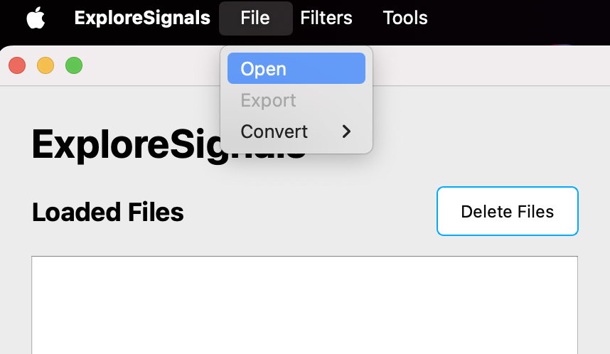
Files can be loaded using the File menu in the menu bar of ExploreSignals. Navigate to File -> Open to open a file browser and select one or multiple ExG files (.csv, .bdf) to load them into the software. The loaded file(s) will appear in the Loaded Files section.
If you are loading Mentalab Explore data from a [...]_ExG.csv file, make sure that the corresponding [...]_Meta.csv file is present in the same folder to ensure the data is loaded correctly. Additionally, if you want to visualize markers alongside the data, make sure that the corresponding [...]_Marker.csv file is present in the same folder.
These files are matched to each other using the file name, so if you need to rename the files (i.e. by exporting filtered data with ExploreSignals), ensure that the file containing EXG data ends in _ExG.csv, the file containing markers ends in _Marker.csv and the file containing the metadata ends in _Meta.csv.
Applying Filters
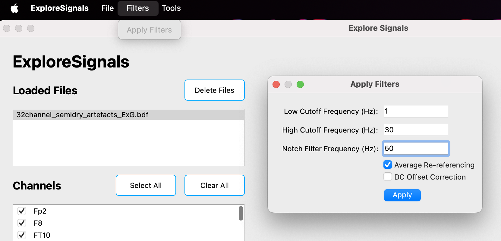
Filters can be applied from the Filters menu in the menu bar. Select the file you want to filter in the Loaded Files section, then navigate to Filters -> Apply Filters to open a pop-up, enter values for the filters you want to use and click on apply to filter the data. The following filters are available:
- High-pass / Low-pass filters
- Notch filter (e.g., to remove 50/60 Hz line noise)
- Re-referencing options
- DC offset correction
The filtered data will be added in the Loaded Files section with its name being made up of the filename of the original file and metadata about the applied filters.
Channel Selection
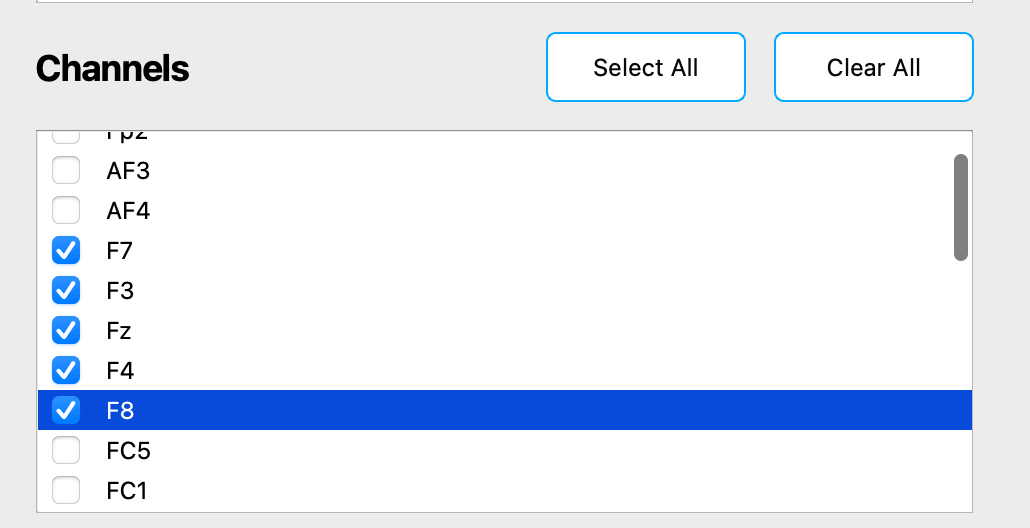
To enable or disable channels for visualization, select a file in the Loaded Files section and check or uncheck channels in the Channels section below before using any of the visualization actions. To quickly enable or disable all channels, you can use the Select All and Clear All buttons above the Channels section.
Visualization Options
Click the corresponding button to visualize the selected data.
Tip: Use the interactive toolbar above the plots to zoom, pan, and explore plots in detail.
- Plot Time Domain – View raw signal over time.
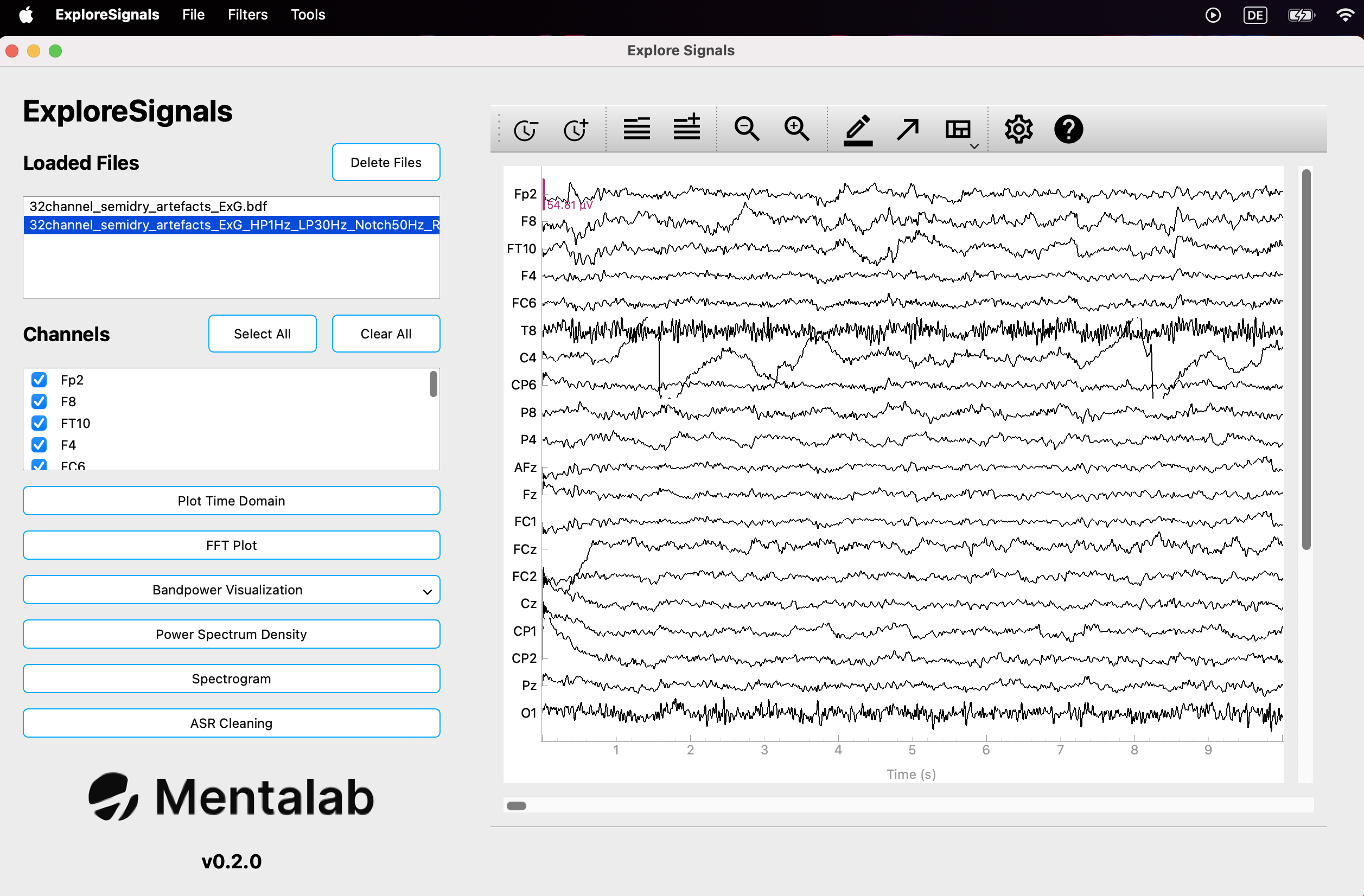
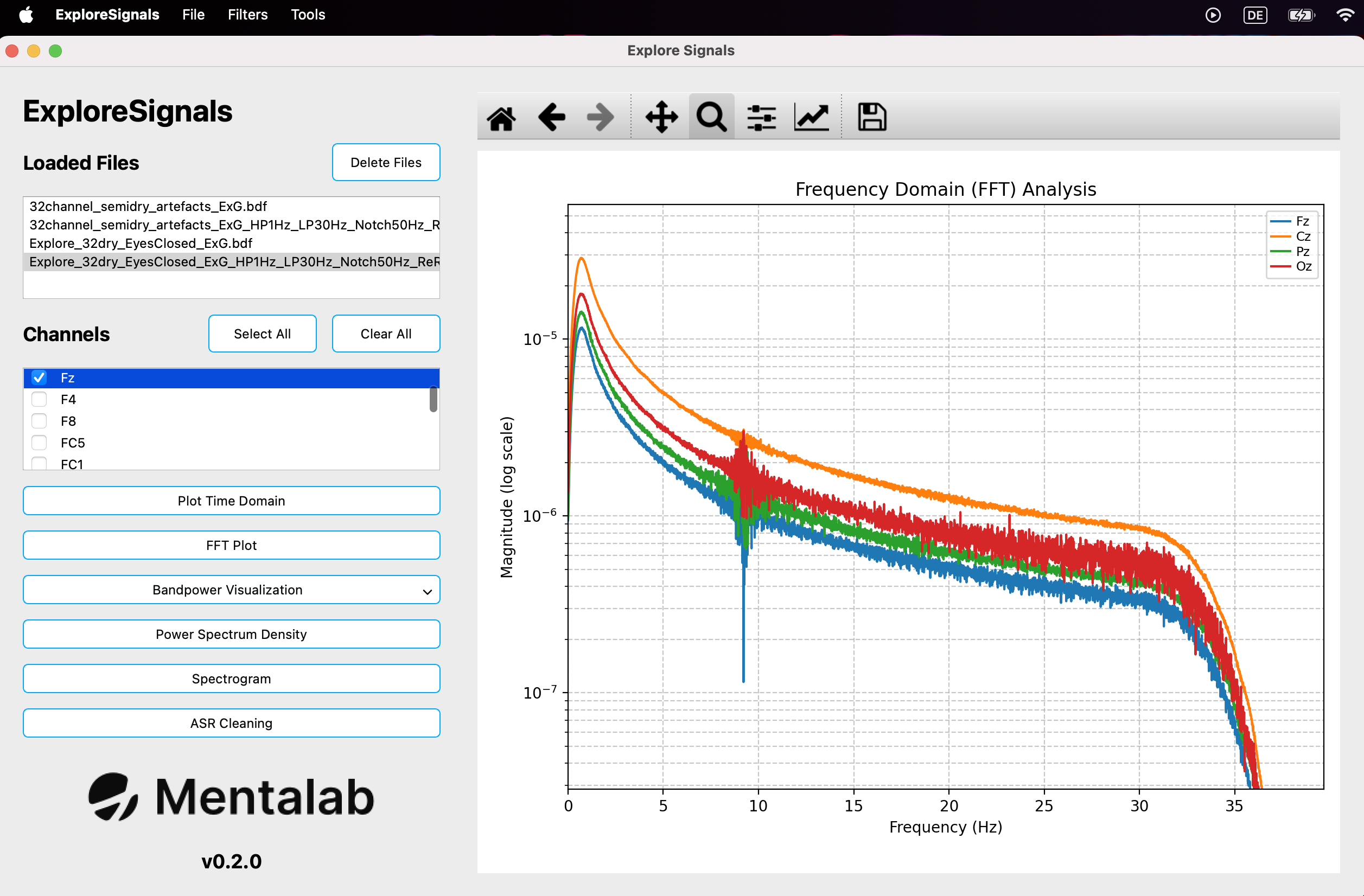
- FFT Plot – Visualize frequency content using Fast Fourier Transform.
-
Bandpower Visualization – Show power in defined frequency bands (delta, theta, alpha, beta, gamma). The plots show the average for the selected channels. When clicking on the Bandpower Visualization button, you have two options to visualize the data.
-
Time Domain - Visualize the power in the frequency bands over time. For this plot, the bandpower is calculated on one second windows with 0.1s between each calculated sample.
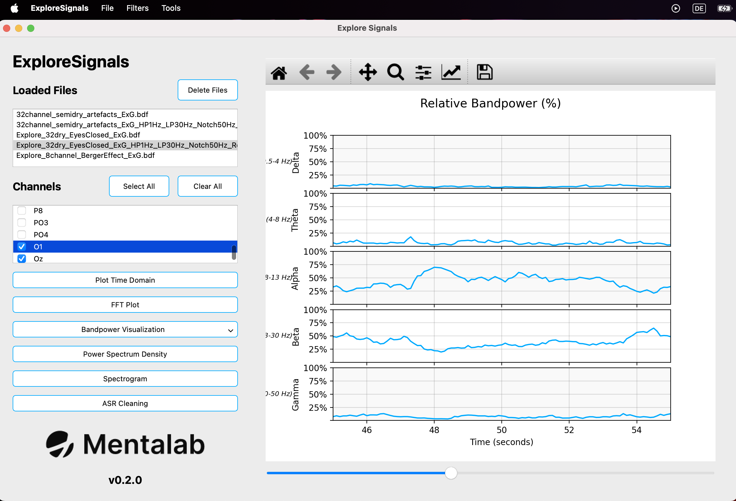
Visualizing the power over time in the different frequency bands of a recording in ExploreSignals. -
Bars - Visualize the power in the frequency bands for the entire recording in a bar plot.
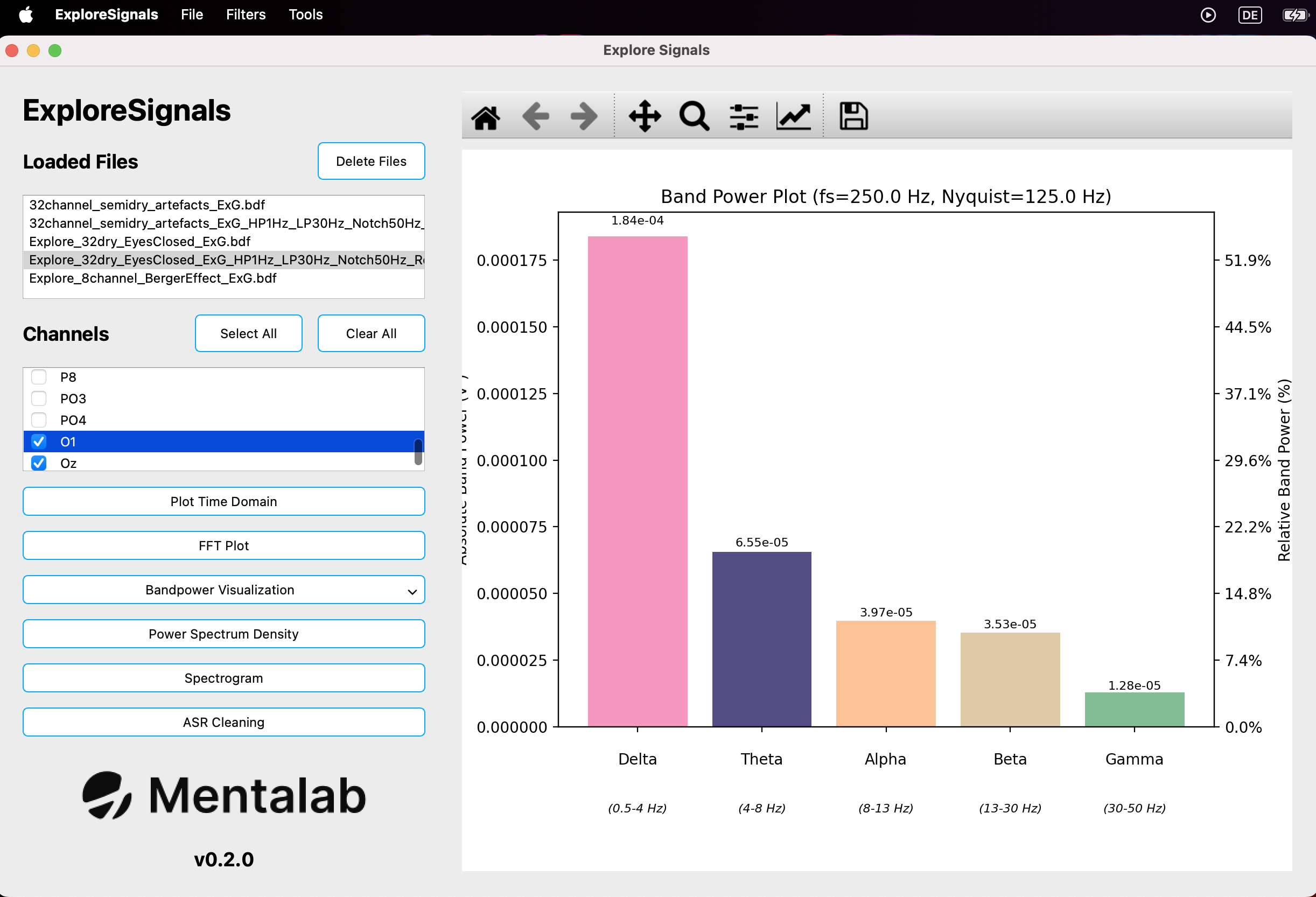
Visualizing the power in the different frequency bands of a recording in a bar plot.
-
-
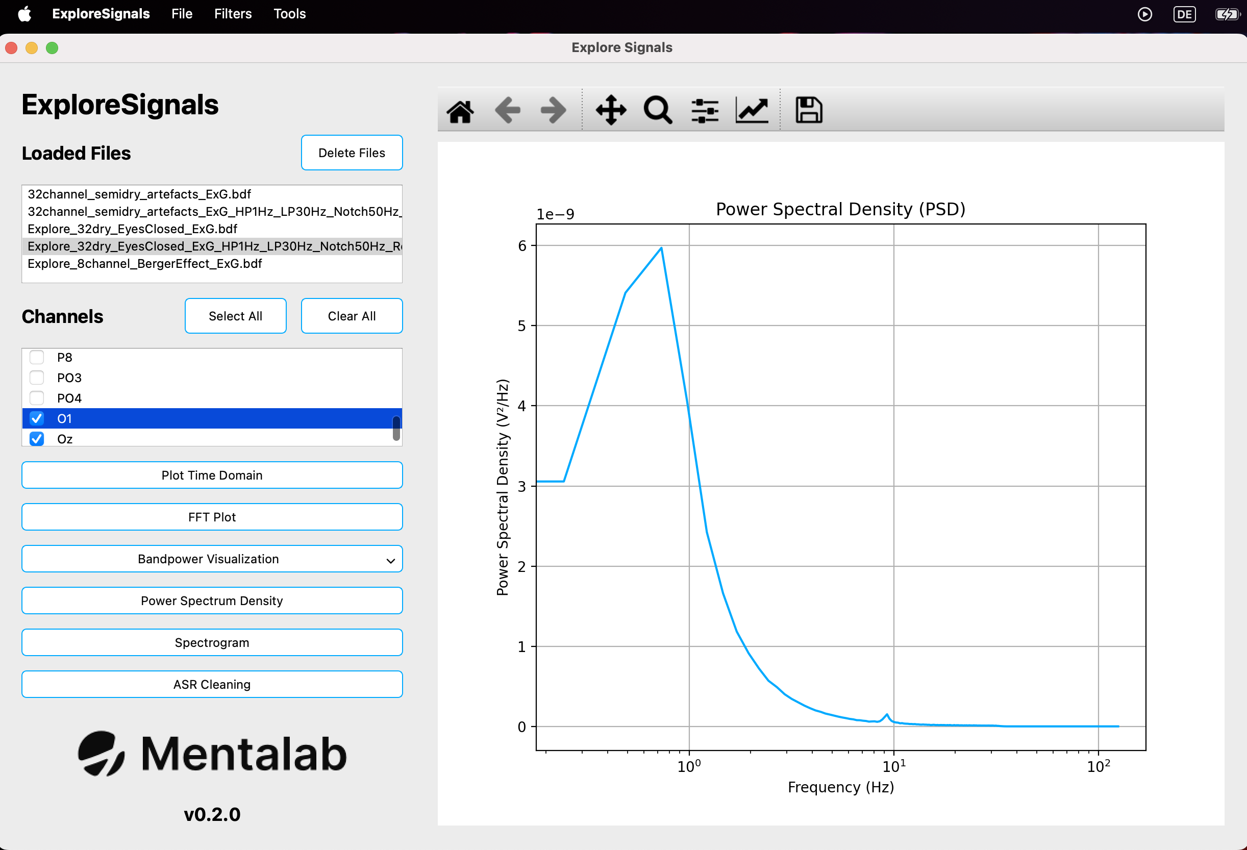
Power Spectrum Density – Analyze power distribution over frequency. The plot shows the average for the selected channels.
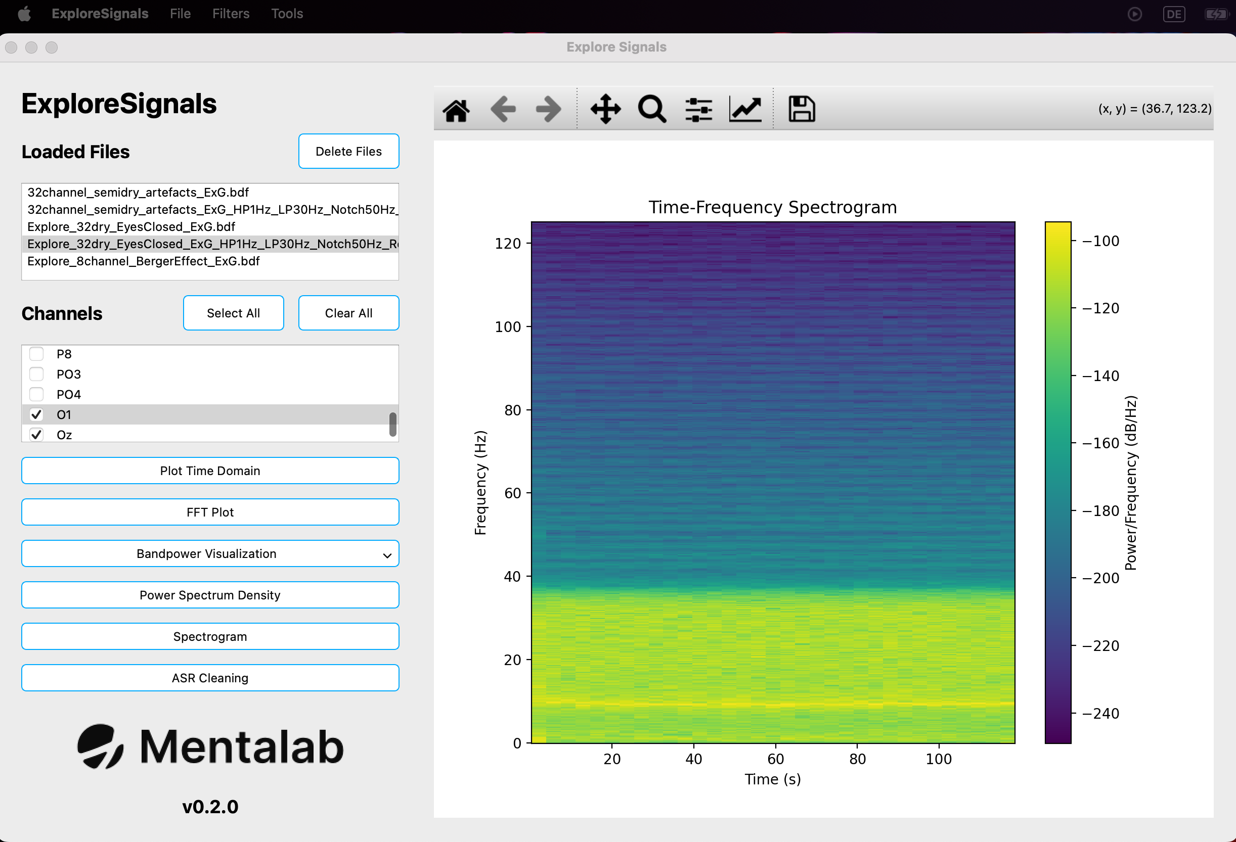
- Spectrogram – Display power as a function of time and frequency. The plot shows the average for the selected channels.
- ASR Cleaning - Apply ASR to the data and visualize the cleaned signal alongside the original signal afterwards. For more details, refer to the section on ASR.
Exporting Data
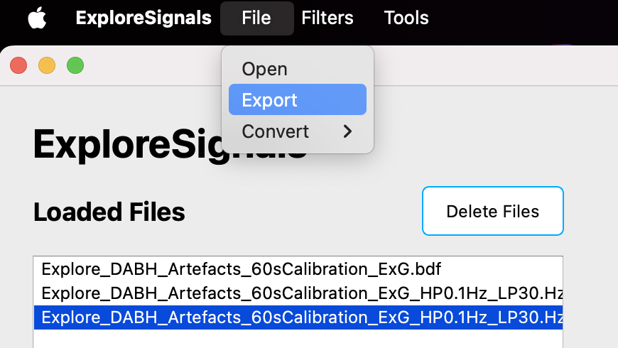
Data (original and processed) can be exported from the File menu in the menu bar. Select the file you want to export in the Loaded Files section, then navigate to File -> Export to open a file browser. In the file browser, you can change the file name and select the file format you want to save the data in (.csv or .bdf).
Artifact Subspace Reconstruction (ASR)
The implementation for ASR is based on (parts of) the open source clean_rawdata plugin for EEGLab (originally written in MATLAB), the code of which can be found in this public repository. You can also find more about ASR by visiting the linked repository and referring to the ReadMe. An even more in-depth discussion on ASR (inlcuding the history of its development) and its validity for artifact removal for EEG data can be found in the wiki of the same repository.
Please make sure to read the linked pages if you are planning to apply ASR and work with the cleaned data, as ASR may come with a possible loss of signal together with removal of artifacts and will perform better on certain types of data.
ASR requires a calibration window to clean the data, this should be a section of the data that has as few artifacts as possible - ideally none. Keep this in mind when selecting the calibration window length and the starting time of the calibration window. Additionally, the algorithm is recommended for EEG signals, the output for other types of biosignals may be a lot worse (i.e. by decreasing signal to noise ratio if more signal than artifacts is removed from the data). Another factor to consider when applying ASR is the number of channels considered. While ASR requires multiple channels to effectively clean signals, it is difficult to recommend a minimum number of channels to be used. Research, however, suggests that “ASR could achieve effective artifact removal for standard 20-channel EEG”1.
Standard deviation cutoff
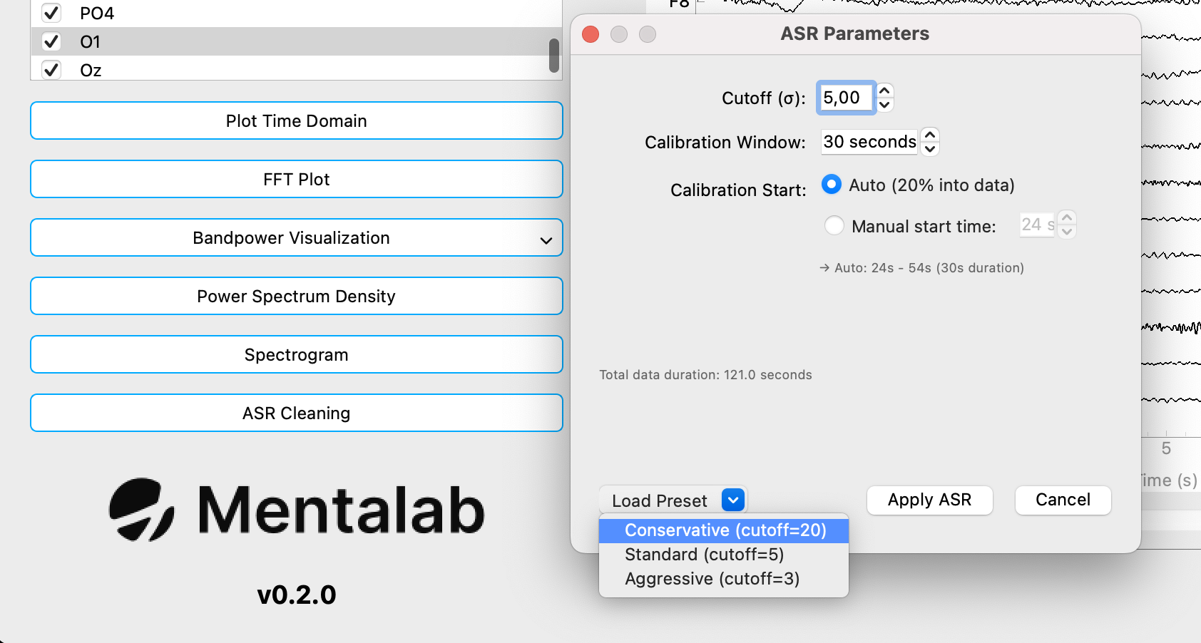
The cutoff field in the ASR pop-up refers to the standard deviation cutoff applied during cleaning. This cutoff determines the thresholds used (relative to the calibration data) for recognizing portions of the data as artifacts. A lower threshold will cause more of the data to be recognized as artifacts while a higher threshold will do the opposite. A cutoff of 3.0 is considered aggressive (and going lower is not recommended and thus blocked by ExploreSignals), 5.0 is the default cutoff in ExploreSignals and 20.0 is considered conservative (and also the default in EEGLab’s clean_rawdata plugin).
Calibration Window
The Calibration Window determines how large the window of data for calibration should be, the default (and minimum!) is 30.0s. Note that the recommended window for a cutoff of 20.0 (the default in clean_rawdata) is 60.0s.
Calibration Start
The Calibration Start determines the beginning of the calibration window. The default is Auto, which automatically places the start of the window at 20% into the recording. As an example, if the recording is 120.0s, the calibration window is set to 30.0s and Auto is selected for the Calibration Start, the calibration window will be from 24.0s to 54.0s. Alternatively, it is also possible to manually choose the start of the calibration window by selecting Manual start time and changing the accompanying field to the starting second.
Applying ASR to a loaded file
In order to clean data using ASR, load a file (as outlined in the section on loading data), select it in the Loaded Files section and click on the ASR Cleaning button. A pop-up will be shown that allows changing the previously mentioned parameters for the algorithm. The button Load Preset can be used to bring up a menu to load recommended presets for the cutoff and accompanying calibration window, available presets are Aggressive (with a cutoff of 3.0 and a calibration window of 30s), Standard (with a cutoff of 5.0 and a calibration window of 30s) and lastly Conservative (with a cutoff of 20.0 and a calibration window of 60s).
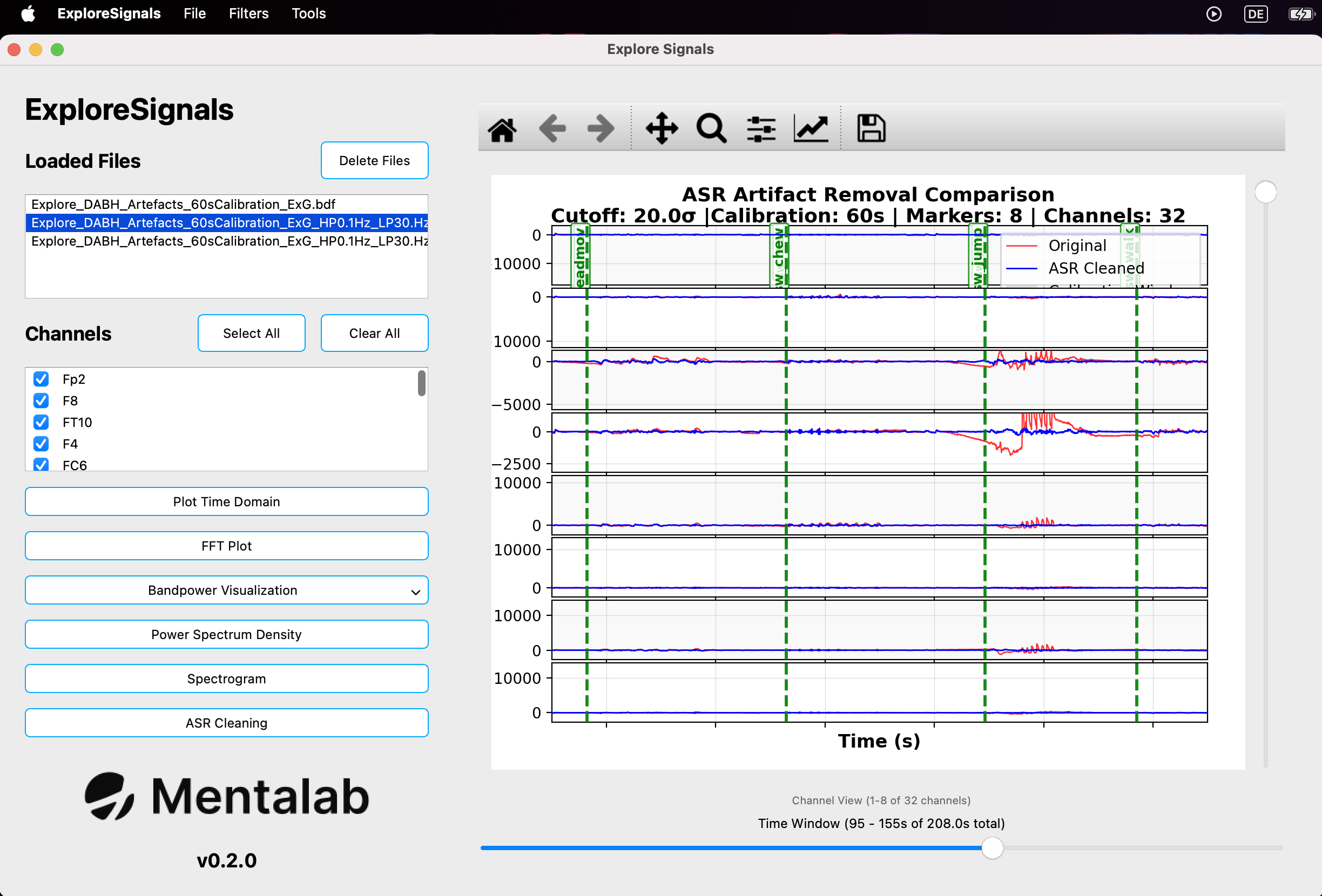
When you are finished with changing the parameters for the algorithm, clicking Apply ASR will clean the data and, once finished, bring up a comparison view of the cleaned data and the original data. Note that the implementation applies a high-pass filter internally to correct for drift and that the resulting cleaned signal will also be zero-mean as a result. If the original data is not filtered and / or zero-mean, the signal may not appear overlayed with / having the same baseline as the cleaned signal.
The cleaned data is added to the list of Loaded Files and can be visualized (and analyzed) the same as other loaded data.
Converting and repairing recordings
Converting to and from .csv and .bdf
To convert an existing recording from .csv to .bdf and vice-versa, you can load the file you want to convert as explained in this section and simply export it to the other format as explained in this section.
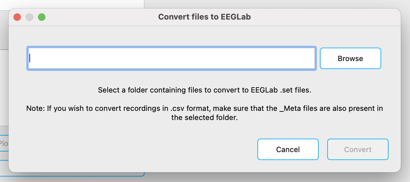
Converting to EEGLab dataset (.set)
Recordings in .csv and .edf/.bdf format can be converted to .set files compatible with Matlab’s EEGLab plugin. You can use this feature by selecting File -> Convert -> Convert files to EEGLab. A pop-up will open to select the folder containing the .edf/.bdf files to convert. The .set files will be created in a subfolder called datasets placed in the selected directory. To convert recordings from .csv format, the respective _Meta.csv file needs to be present in same folder.
Converting from .BIN
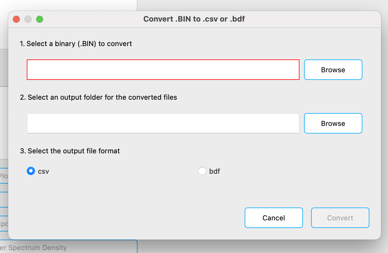
You can convert the binary files from the Explore device’s internal memory (.BIN) to .csv or .bdf files. To do so, select File -> Convert -> Convert .BIN to .csv or .bdf. This will open a pop-up to select the file to convert, the folder to save the converted files to and the output file format.
Converting to .csv generates four files: ExG, orientation, marker and metadata ([...]_ExG.csv, [...]_ORN.csv, [...]_Marker.csv and [...]_Meta.csv).
Converting to .bdf generates two files: ExG and orientation ([...]_ExG.bdf and [...]_ORN.bdf) - markers will be written to the ExG file. Note that the data is written in BDF+ format (using 24-bit resolution, as opposed to EDF/EDF+)
.csv/.bdf file for the ExG data with the given file name plus the time the setting changed.
Repairing .csv recordings
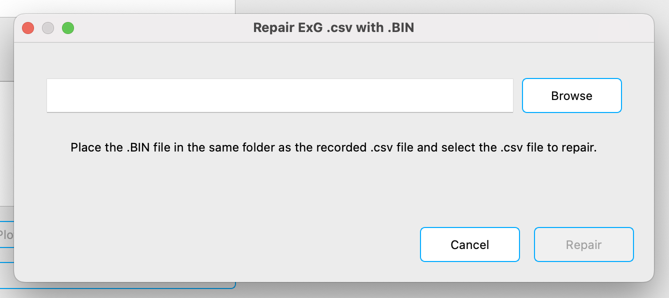
If some packets are dropped during recording with explorepy or Explore Desktop, the binary file from the Explore device can be used to repair the recorded .csv file. To repair a recorded .csv file, select Tools -> Repair ExG .csv with .BIN. This will open a pop-up that lets you select a .csv file to repair. To repair the selected file, make sure it is located in the same folder as the respective .BIN file that should be used to repair it before clicking on the Repair button. The repaired file will be place inside the same folder as the file that was selected. It will be named like the selected file but with _recovered_ExG added to the file name.
For more information or support, do not hesitate to get in contact at: support@mentalab.com
-
Chang, Chi-Yuan, et al. “Evaluation of artifact subspace reconstruction for automatic artifact components removal in multi-channel EEG recordings.” IEEE transactions on biomedical engineering 67.4 (2019): 1114-1121. ↩︎